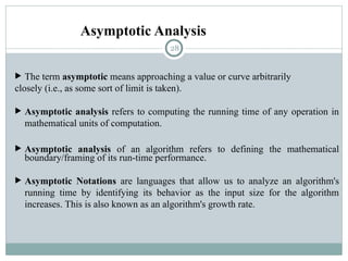
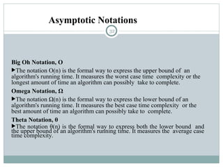
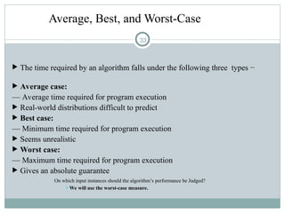
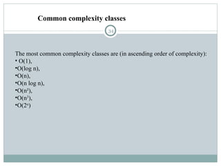
JIMMA UNIVERSITY
JIMMA INSTITUTE OF TECHNOLOGY
FACULTY OF COMPUTING AND INFORMATICS
CHAPTER ONE
Data structures and algorithms
1
Introduction to Data
Structures and Algorithms
Objective
Data structures and algorithms
2
At the end of the session, students should have a basic
understanding of
Data structure
Classification of data structure
Algorithm
Characteristics of algorithms
Algorithm analysis
Introduction to Data structures and Algorithms
Data structures and algorithms
 Program = Algorithm + Data structure
Data Structure:
 The way data is organized in a computer’s memory so
that it can be used effectively.
Algorithm :
 The sequence of computational steps to solve a
problem.
3
Cont’d
Data structures and algorithms
 All of you have programmed;
 already been exposed to algorithms and data structure.
 Perhaps
 you didn't see them as separate entities;
 you saw data structures as simple programming constructs
(provided by STL--standard template library).
 However, data structures are quite distinctfrom
algorithms, and very important in their own right.
4
Why Are Data Structures and Algorithms So
Important?
Data structures and algorithms
 Data structure and algorithms are two of the most important
aspects of computer science.
 Data structures allow us to organize and store data, while
algorithms allow us to process that data in a meaningful way.
 Learning data structure and algorithms will help you become a
better programmer.
 You will be able to write code that is more efficient and more
reliable.
 You will also be able to solve problems more quickly and more
effectively.
5
Cont’d
Data structures and algorithms
6
 Model
 defines an abstract view to the problem
 define the properties of the problem
 Properties of the problem include
 The data which are affected and
 The operations that are involved in the problem.
 is an abstraction of a data structure which provides only
the interface to which a data structure must follow.
 The interface doesn’t give any specific details about
how something should be implemented or in what
programming language.
Abstract Data Type
7
Data structures and algorithms
Cont’d
Data structures and algorithms
 Consists of an abstract data structure and operations
 Specifies:
 What can be stored in the ADT
 What operations can be done on/by the ADT
 E.g., if we are going to model employees of an organization:
 ADT stores employees with
their relevant attributes and
discarding irrelevant attributes.
 ADT supports
hiring, firing, retiring, … operations.
8
Data structure (DS)
Data structures and algorithms
is a language construct that the programmer has defined in order to implement
an abstract data type.
There are lots of formalized and standard Abstract data types
 such as Stacks, Queues, Trees, etc.
Do all characteristics need to be modeled?
Not at all it depends on
 the scope of the model
 the reason for developing the model
Abstraction
is a process of classifying characteristics as relevant and irrelevant for the
particular purpose at hand and ignoring the irrelevant ones.
9
CLASSIFICATION OF DATA STRUCTURE
 What is data structure
 is basically a technique of organizing and storing of
different types of data items in computer memory.
 It is considered as not only the storing of data
elements but also the maintaining of the logical
relationship existing between individual data
elements.
10
Data structures and algorithms
CLASSIFICATION OF DATA STRUCTURE
Data structures and algorithms
11
1. Primitive data structure
2. Non-primitive data structure
Cont’d
Data structures and algorithms
 Primitive data structure:
 also known as basic data structures.
 predefined types of data, which are supported by the
programming language.
 Non-Primitive data structure:
 are highly developed complex data structures.
 are not defined by the programming language, but are instead
created by the programmer.
 Are responsible for organizing the group of homogeneous and
heterogeneous data elements.
12
Cont’d
Data structures and algorithms
The linear and non-linear data structure are the
subclassification of non-primitive data structure.
Difference:
 Linear data structure arranges the data into a
sequence and follow some sort of order.
Non-linear data structure does not organize the
data in a sequential manner.
13
Algorithm
Data structures and algorithms
 An algorithm can be thought of as a set of instructions that specifies
how to solve a particular problem.
 is a well-defined computational procedure that takes some value or a
set of values as input and produces some value or a set of values as
output
 An algorithm transforms data structures from one state to another state
in two ways:
 An algorithm may change the value held by a data structure
 An algorithm may change the data structure itself
14
Properties of algorithm
Data structures and algorithms
 Finiteness :-Algorithms must terminate after a finite number of steps.
 Definiteness :- Each instruction of the algorithm should be clear and unambiguous.
 Sequence :-Should be written in sequence
 Feasibility :-Should be feasible with the available resources.
 Correctness: It should produce the correct output.
 Language Independent
 An algorithm must be language-independent, which means that its
instructions can be implemented in any language and produce the
same results.
15
Algorithm Analysis
Data structures and algorithms
 Refers to the process of determining the amount of computing
time and storage space required by different algorithms.
 A process of predicting the resource requirement of algorithms
in a given environment.
 Main resources are:
Running Time
Memory Usage
Communication Bandwidth
16
Approaches to measure the efficiency of algorithms
Data structures and algorithms
 Empirical:
 competing algorithms and trying them on different
instances.
 It uses actual clock-time.
 Theoretical:
 Determining the quantity of resources required
mathematically (Execution time, memory space, etc.) needed
by each algorithm.
17
Cont’d
Data structures and algorithms
18
 However, it is difficult to use actual clock-time as a consistent
measure of an algorithm‘s efficiency, because clock-time can
vary based on many things. For example,
 Specific processor speed, Current processor
load
 Specific data for a particular run of the program
Input Size, Input Properties
 Operating Environment
Complexity Analysis
 Is the systematic study of the cost of computation, measured
either
 in time units or
 in operations performed, or
 in the amount of storage space required
The goal is to have a meaningful measure that permits
comparison of algorithms independent of operating platform.
19
Cont‘d
Two things to consider:
 Time Complexity:
 Determine the approximate number of operations required to
solve a problem of size n.
 Space Complexity:
Determine the approximate memory required to solve a problem
of size n.
20
Benefits
 Provides the short hand method, to find how much time
algorithm takes (approx.)
 Its useful way of estimating the efficiency of an algorithm, without having to
measure actual run times.
 Gives the choice to select among the best algorithms
available
21
Analysis Rules:
1. We assume an arbitrary time unit.
2. Execution of one of the following operations takes time 1:
• Assignment Operation
• Single Input/output Operation
• Single Boolean Operations
• Single Arithmetic Operations
• Function Return
22
Cont’d
3. Running time of a selection statement (if, switch)
is the time for the condition evaluation +
the maximum running times for the individual clauses in the
selection.
23
Cont‘d
4. Loops: The running time for a loop is equal to
the running time for the statements inside the
loop * number of iterations.
Remark:
The total running time of a statement inside a
group of nested loops is
 The running time of the statements multiplied by the
product of the sizes of all the loops.
For nested loops, analyze inside out.
Always assume that the loop executes the maximum number of iterations
possible.
24
Cont’d
5. The running time of a function call is
1 for setup +
the time for any parameter calculations +
the time required for the execution of the function body.
25
Example
int count()
{
int k=0;
cout<< “Enter an
integer”;
cin>>n;
for (i=0;i<n;i++)
k=k+1;
return 0;
}
T (n)= 1+1+1+(1+n+1+n)+2n+1 = 4n+6 = O(n)
In the for loop:
• 1 assignment, n+1 tests, and n
increments.
• n loops of 2 units for an assignment,
and an addition.
• 1 for the return statement.
Time Units to Compute
-------------------------------------------------
•1 for the assignment statement: int
k=0
•1 for the output statement.
•1 for the input statement.
26
void func()
{
int x=0; int i=0;
int j=1;
cout<< ―Enter an Integer
value ; cin>>n;
‖
while (i<n){ x++;
i++; }
while (j<n) {
j++;
} }
Time Units to Compute
-------------------------------------------------
1 for the first assignment statement: x=0;
1 for the second assignment statement: i=0;
1 for the third assignment statement: j=1;
1 for the output statement. 1 for the input
statement.
In the first while loop:
n+1 tests
n loops of 2 units for the two increment
(addition) operations
In the second while loop:
n tests
n-1 increments
------------------------------------------------------
-
T (n)= 1+1+1+1+1+n+1+2n+n+n-1 = 5n+5
= O(n)
Example
27
Asymptotic Analysis
 The term asymptotic means approaching a value or curve arbitrarily
closely (i.e., as some sort of limit is taken).
 Asymptotic analysis refers to computing the running time of any operation in
mathematical units of computation.
 Asymptotic analysis of an algorithm refers to defining the mathematical
boundary/framing of its run-time performance.
 Asymptotic Notations are languages that allow us to analyze an algorithm's
running time by identifying its behavior as the input size for the algorithm
increases. This is also known as an algorithm's growth rate.
28
Simplifying the Bound
 T(n) = ck nk + ck-1 nk-1 + ck-2 nk-2 + … + c1 n +
co
 too complicated
 too many terms
 Difficult to compare two expressions, each with 10 or
20 terms
 Do we really need that many terms?
29
Simplifications
 Keep just one term!
 the fastest growing term (dominates the runtime)
 No constant coefficients are kept
 Constant coefficients affected by machines, languages, etc.
 Asymptotic behavior (as n gets large) is determined
entirely by the leading term.
 Example. T(n) = 10 n3 + n2 + 40n + 800
If n = 1,000, thenT(n) = 10,001,040,800
error is 0.01% if we drop all but the n3 term
30
T(n) keep one drop coef
3n2
+4n+1 3 n2
n2
101 n2
+102 101 n2
n2
15 n2+6n 15 n2
n2
a n2+bn+c a n2
n2
Asymptotic
 They all have the same “growth” rate
31
Asymptotic Notations
Big Oh Notation, Ο
The notation Ο(n) is the formal way to express the upper bound of an
algorithm's running time. It measures the worst case time complexity or the
longest amount of time an algorithm can possibly take to complete.
Omega Notation, Ω
The notation Ω(n) is the formal way to express the lower bound of an
algorithm's running time. It measures the best case time complexity or the
best amount of time an algorithm can possibly take to complete.
Theta Notation, θ
The notation θ(n) is the formal way to express both the lower bound and
the upper bound of an algorithm's running time. It measures the average case
time complexity.
32
Average, Best, and Worst-Case
 The time required by an algorithm falls under the following three types −
 Average case:
— Average time required for program execution
 Real-world distributions difficult to predict
 Best case:
— Minimum time required for program execution
 Seems unrealistic
 Worst case:
— Maximum time required for program execution
 Gives an absolute guarantee
On which input instances should the algorithm’s performance be Judged?
We will use the worst-case measure.
33
Common complexity classes
34
The most common complexity classes are (in ascending order of complexity):
• O(1),
•O(log n),
•O(n),
•O(n log n),
•O(n²),
•O(n3
),
•O(2n
)
The end of
chapter one
35

assignment character education assignment

  • 1.
    JIMMA UNIVERSITY JIMMA INSTITUTEOF TECHNOLOGY FACULTY OF COMPUTING AND INFORMATICS CHAPTER ONE Data structures and algorithms 1 Introduction to Data Structures and Algorithms
  • 2.
    Objective Data structures andalgorithms 2 At the end of the session, students should have a basic understanding of Data structure Classification of data structure Algorithm Characteristics of algorithms Algorithm analysis
  • 3.
    Introduction to Datastructures and Algorithms Data structures and algorithms  Program = Algorithm + Data structure Data Structure:  The way data is organized in a computer’s memory so that it can be used effectively. Algorithm :  The sequence of computational steps to solve a problem. 3
  • 4.
    Cont’d Data structures andalgorithms  All of you have programmed;  already been exposed to algorithms and data structure.  Perhaps  you didn't see them as separate entities;  you saw data structures as simple programming constructs (provided by STL--standard template library).  However, data structures are quite distinctfrom algorithms, and very important in their own right. 4
  • 5.
    Why Are DataStructures and Algorithms So Important? Data structures and algorithms  Data structure and algorithms are two of the most important aspects of computer science.  Data structures allow us to organize and store data, while algorithms allow us to process that data in a meaningful way.  Learning data structure and algorithms will help you become a better programmer.  You will be able to write code that is more efficient and more reliable.  You will also be able to solve problems more quickly and more effectively. 5
  • 6.
    Cont’d Data structures andalgorithms 6  Model  defines an abstract view to the problem  define the properties of the problem  Properties of the problem include  The data which are affected and  The operations that are involved in the problem.
  • 7.
     is anabstraction of a data structure which provides only the interface to which a data structure must follow.  The interface doesn’t give any specific details about how something should be implemented or in what programming language. Abstract Data Type 7 Data structures and algorithms
  • 8.
    Cont’d Data structures andalgorithms  Consists of an abstract data structure and operations  Specifies:  What can be stored in the ADT  What operations can be done on/by the ADT  E.g., if we are going to model employees of an organization:  ADT stores employees with their relevant attributes and discarding irrelevant attributes.  ADT supports hiring, firing, retiring, … operations. 8
  • 9.
    Data structure (DS) Datastructures and algorithms is a language construct that the programmer has defined in order to implement an abstract data type. There are lots of formalized and standard Abstract data types  such as Stacks, Queues, Trees, etc. Do all characteristics need to be modeled? Not at all it depends on  the scope of the model  the reason for developing the model Abstraction is a process of classifying characteristics as relevant and irrelevant for the particular purpose at hand and ignoring the irrelevant ones. 9
  • 10.
    CLASSIFICATION OF DATASTRUCTURE  What is data structure  is basically a technique of organizing and storing of different types of data items in computer memory.  It is considered as not only the storing of data elements but also the maintaining of the logical relationship existing between individual data elements. 10 Data structures and algorithms
  • 11.
    CLASSIFICATION OF DATASTRUCTURE Data structures and algorithms 11 1. Primitive data structure 2. Non-primitive data structure
  • 12.
    Cont’d Data structures andalgorithms  Primitive data structure:  also known as basic data structures.  predefined types of data, which are supported by the programming language.  Non-Primitive data structure:  are highly developed complex data structures.  are not defined by the programming language, but are instead created by the programmer.  Are responsible for organizing the group of homogeneous and heterogeneous data elements. 12
  • 13.
    Cont’d Data structures andalgorithms The linear and non-linear data structure are the subclassification of non-primitive data structure. Difference:  Linear data structure arranges the data into a sequence and follow some sort of order. Non-linear data structure does not organize the data in a sequential manner. 13
  • 14.
    Algorithm Data structures andalgorithms  An algorithm can be thought of as a set of instructions that specifies how to solve a particular problem.  is a well-defined computational procedure that takes some value or a set of values as input and produces some value or a set of values as output  An algorithm transforms data structures from one state to another state in two ways:  An algorithm may change the value held by a data structure  An algorithm may change the data structure itself 14
  • 15.
    Properties of algorithm Datastructures and algorithms  Finiteness :-Algorithms must terminate after a finite number of steps.  Definiteness :- Each instruction of the algorithm should be clear and unambiguous.  Sequence :-Should be written in sequence  Feasibility :-Should be feasible with the available resources.  Correctness: It should produce the correct output.  Language Independent  An algorithm must be language-independent, which means that its instructions can be implemented in any language and produce the same results. 15
  • 16.
    Algorithm Analysis Data structuresand algorithms  Refers to the process of determining the amount of computing time and storage space required by different algorithms.  A process of predicting the resource requirement of algorithms in a given environment.  Main resources are: Running Time Memory Usage Communication Bandwidth 16
  • 17.
    Approaches to measurethe efficiency of algorithms Data structures and algorithms  Empirical:  competing algorithms and trying them on different instances.  It uses actual clock-time.  Theoretical:  Determining the quantity of resources required mathematically (Execution time, memory space, etc.) needed by each algorithm. 17
  • 18.
    Cont’d Data structures andalgorithms 18  However, it is difficult to use actual clock-time as a consistent measure of an algorithm‘s efficiency, because clock-time can vary based on many things. For example,  Specific processor speed, Current processor load  Specific data for a particular run of the program Input Size, Input Properties  Operating Environment
  • 19.
    Complexity Analysis  Isthe systematic study of the cost of computation, measured either  in time units or  in operations performed, or  in the amount of storage space required The goal is to have a meaningful measure that permits comparison of algorithms independent of operating platform. 19
  • 20.
    Cont‘d Two things toconsider:  Time Complexity:  Determine the approximate number of operations required to solve a problem of size n.  Space Complexity: Determine the approximate memory required to solve a problem of size n. 20
  • 21.
    Benefits  Provides theshort hand method, to find how much time algorithm takes (approx.)  Its useful way of estimating the efficiency of an algorithm, without having to measure actual run times.  Gives the choice to select among the best algorithms available 21
  • 22.
    Analysis Rules: 1. Weassume an arbitrary time unit. 2. Execution of one of the following operations takes time 1: • Assignment Operation • Single Input/output Operation • Single Boolean Operations • Single Arithmetic Operations • Function Return 22
  • 23.
    Cont’d 3. Running timeof a selection statement (if, switch) is the time for the condition evaluation + the maximum running times for the individual clauses in the selection. 23
  • 24.
    Cont‘d 4. Loops: Therunning time for a loop is equal to the running time for the statements inside the loop * number of iterations. Remark: The total running time of a statement inside a group of nested loops is  The running time of the statements multiplied by the product of the sizes of all the loops. For nested loops, analyze inside out. Always assume that the loop executes the maximum number of iterations possible. 24
  • 25.
    Cont’d 5. The runningtime of a function call is 1 for setup + the time for any parameter calculations + the time required for the execution of the function body. 25
  • 26.
    Example int count() { int k=0; cout<<“Enter an integer”; cin>>n; for (i=0;i<n;i++) k=k+1; return 0; } T (n)= 1+1+1+(1+n+1+n)+2n+1 = 4n+6 = O(n) In the for loop: • 1 assignment, n+1 tests, and n increments. • n loops of 2 units for an assignment, and an addition. • 1 for the return statement. Time Units to Compute ------------------------------------------------- •1 for the assignment statement: int k=0 •1 for the output statement. •1 for the input statement. 26
  • 27.
    void func() { int x=0;int i=0; int j=1; cout<< ―Enter an Integer value ; cin>>n; ‖ while (i<n){ x++; i++; } while (j<n) { j++; } } Time Units to Compute ------------------------------------------------- 1 for the first assignment statement: x=0; 1 for the second assignment statement: i=0; 1 for the third assignment statement: j=1; 1 for the output statement. 1 for the input statement. In the first while loop: n+1 tests n loops of 2 units for the two increment (addition) operations In the second while loop: n tests n-1 increments ------------------------------------------------------ - T (n)= 1+1+1+1+1+n+1+2n+n+n-1 = 5n+5 = O(n) Example 27
  • 28.
    Asymptotic Analysis  Theterm asymptotic means approaching a value or curve arbitrarily closely (i.e., as some sort of limit is taken).  Asymptotic analysis refers to computing the running time of any operation in mathematical units of computation.  Asymptotic analysis of an algorithm refers to defining the mathematical boundary/framing of its run-time performance.  Asymptotic Notations are languages that allow us to analyze an algorithm's running time by identifying its behavior as the input size for the algorithm increases. This is also known as an algorithm's growth rate. 28
  • 29.
    Simplifying the Bound T(n) = ck nk + ck-1 nk-1 + ck-2 nk-2 + … + c1 n + co  too complicated  too many terms  Difficult to compare two expressions, each with 10 or 20 terms  Do we really need that many terms? 29
  • 30.
    Simplifications  Keep justone term!  the fastest growing term (dominates the runtime)  No constant coefficients are kept  Constant coefficients affected by machines, languages, etc.  Asymptotic behavior (as n gets large) is determined entirely by the leading term.  Example. T(n) = 10 n3 + n2 + 40n + 800 If n = 1,000, thenT(n) = 10,001,040,800 error is 0.01% if we drop all but the n3 term 30
  • 31.
    T(n) keep onedrop coef 3n2 +4n+1 3 n2 n2 101 n2 +102 101 n2 n2 15 n2+6n 15 n2 n2 a n2+bn+c a n2 n2 Asymptotic  They all have the same “growth” rate 31
  • 32.
    Asymptotic Notations Big OhNotation, Ο The notation Ο(n) is the formal way to express the upper bound of an algorithm's running time. It measures the worst case time complexity or the longest amount of time an algorithm can possibly take to complete. Omega Notation, Ω The notation Ω(n) is the formal way to express the lower bound of an algorithm's running time. It measures the best case time complexity or the best amount of time an algorithm can possibly take to complete. Theta Notation, θ The notation θ(n) is the formal way to express both the lower bound and the upper bound of an algorithm's running time. It measures the average case time complexity. 32
  • 33.
    Average, Best, andWorst-Case  The time required by an algorithm falls under the following three types −  Average case: — Average time required for program execution  Real-world distributions difficult to predict  Best case: — Minimum time required for program execution  Seems unrealistic  Worst case: — Maximum time required for program execution  Gives an absolute guarantee On which input instances should the algorithm’s performance be Judged? We will use the worst-case measure. 33
  • 34.
    Common complexity classes 34 Themost common complexity classes are (in ascending order of complexity): • O(1), •O(log n), •O(n), •O(n log n), •O(n²), •O(n3 ), •O(2n )
  • 35.

Editor's Notes

  • #3 A computer program is a collection of instructions that can be executed by a computer to perform a specific task.
  • #7 Abstraction (from the Latin abs, meaning away from and trahere , meaning to draw) is the process of taking away or removing characteristics from something in order to reduce it to a set of essential characteristics