

![Data Quality 2.0
KDD Tutorial / © 2021 IBM Corporation
Why is automated data quality analysis important?
Lot of progress in last several years on improving ML algorithms and building
automated machine learning toolkits (AutoML) [*]
Several commercially ready pipelines are available
AutoAI with IBM Watson Studio
CloudAutoML from Google
…
Open source pipelines
Autosklearn
Autokeras
…
However, quality of model is upper bounded by quality of input data
GAP: No systematic efforts to measure the quality of data for machine learning (ML)
George Fuechsel,
IBM 305 RAMAC
technician](https://image.slidesharecdn.com/kdd2021tutorialfinal-210820164241/85/Data-Quality-for-Machine-Learning-Tasks-7-320.jpg)


![Filter Based Approaches
On the labeling correctness in
computer vision datasets
[ARK18]
Published in Interactive
Adaptive Learning 2018
Train CNN ensembles to
detect incorrect labels
Voting schemes used:
Majority Voting
KDD Tutorial / © 2021 IBM Corporation
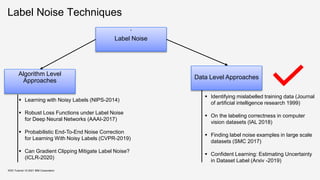
Identifying mislabelled training
data [BF99]
Published in Journal of
artificial intelligence research,
1999
Train filters on parts of the
training data in order to
identify mislabeled examples
in the remaining training data.
Voting schemes used:
Majority Voting
Consensus Voting
Finding label noise examples in large
scale datasets [EGH17]
Published in International
Conference on Systems, Man, and
Cybernetics, 2017
Two-level approach
Level 1 – Train SVM on the
unfiltered data. All support
vectors can be potential
candidates for noisy points.
Level 2 – Train classifier on the
original data without the support
vectors. Samples for which the
original and the predicted label
does not match, are marked as
label noise.
Source: Broadley et al, 1999, Identifying mislabeled training Data](https://image.slidesharecdn.com/kdd2021tutorialfinal-210820164241/85/Data-Quality-for-Machine-Learning-Tasks-25-320.jpg)
![Confident Learning: Estimating
Uncertainty in Dataset Label -2019
The Principles of Confident Learning
Prune to search for label errors
Count to train on clean data
Rank which examples to use during training
KDD Tutorial / © 2021 IBM Corporation
Source: Northcutt et al, 2019. Confident Learning: Estimating Uncertainty in Dataset Label
[NJC19]](https://image.slidesharecdn.com/kdd2021tutorialfinal-210820164241/85/Data-Quality-for-Machine-Learning-Tasks-26-320.jpg)
![KDD Tutorial / © 2021 IBM Corporation
Confident Learning: Estimating
Uncertainty in Dataset Label -2019
Source: Northcutt et al, 2019. Confident Learning: Estimating Uncertainty in Dataset Label
[NJC19]](https://image.slidesharecdn.com/kdd2021tutorialfinal-210820164241/85/Data-Quality-for-Machine-Learning-Tasks-27-320.jpg)
![Data Quality for AI: Label Purity
KDD Tutorial / © 2021 IBM Corporation
Label purity algorithm is built on top of the confident learning-based approach
(CleanLab).
One limitation of CleanLab approach is that it can tag some correct samples as noisy if
they lie in the overlap region thereby generating false positives.
An overlap region is a region where samples of multiple classes start sharing features
because of multiple reasons such as the presence of weak features, fine-grained
classes, etc. This paper improvise the label purity algorithm to address this problem in
two ways:
Algorithm to detect overlap regions, which helps in removing the false positives
Provide an effective neighborhood based pruning mechanism to remove identified
noisy candidate samples
[DQT21]](https://image.slidesharecdn.com/kdd2021tutorialfinal-210820164241/85/Data-Quality-for-Machine-Learning-Tasks-28-320.jpg)
![Data Quality for AI: Label Purity
KDD Tutorial / © 2021 IBM Corporation
Comparison of (a) Precision and (b) Recall of Label Purity Algorithm with CleanLab Algorithm on 35 Datasets
Takeaways:
This algorithm outperforms CleanLab in terms of precision (5−15% improvement).
For recall, both the algorithms have similar performance.
On an average over 35 datasets, (a) the precision of this algorithm is .92 and CleanLab is .76, (b) the recall of this algorithm is
.75 and CleanLab is .78
Overall, 5−16% improvement in precision at the cost of 2% drop in the recall
[DQT21]](https://image.slidesharecdn.com/kdd2021tutorialfinal-210820164241/85/Data-Quality-for-Machine-Learning-Tasks-29-320.jpg)

![Class Overlap : Data Quality for AI
KDD Tutorial / © 2021 IBM Corporation
Analyse the dataset to find samples that reside in
the overlapping region of the data space.
Identify data points which are close to
each other but belongs to
different classes
Identify data points which lies closer to
or other side of the class boundary
Why is it useful for ML pipeline?
Overlapping regions are hard to detect and
can cause ML classifiers to misclassify points
in that region.
If amount of overlap is high, we need good
feature representation or more complex model
Example 2
Example 1
[DQT21]](https://image.slidesharecdn.com/kdd2021tutorialfinal-210820164241/85/Data-Quality-for-Machine-Learning-Tasks-31-320.jpg)
![Data Quality for AI - Class Overlap
KDD Tutorial / © 2021 IBM Corporation
Precision and Recall of Class Overlap Algorithm on 20 datasets (after inducing 30% overlap points)
[DQT21]](https://image.slidesharecdn.com/kdd2021tutorialfinal-210820164241/85/Data-Quality-for-Machine-Learning-Tasks-32-320.jpg)
![Class Overlap : Data Quality for AI
KDD Tutorial / © 2021 IBM Corporation
[DQT21]](https://image.slidesharecdn.com/kdd2021tutorialfinal-210820164241/85/Data-Quality-for-Machine-Learning-Tasks-33-320.jpg)
![Class Overlap
KDD Tutorial / © 2021 IBM Corporation
[XHJ10]
The objective of Support Vector Data Description
(SVDD) is to find a sphere or domain with minimum
volume containing all or most of the data.
The data dropped in both two spheres can be
thought as the overlapping data which is close to or
overlaps with each other.](https://image.slidesharecdn.com/kdd2021tutorialfinal-210820164241/85/Data-Quality-for-Machine-Learning-Tasks-34-320.jpg)

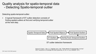
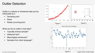
![Outlier Detection
KDD Tutorial / © 2021 IBM Corporation
[OT21]](https://image.slidesharecdn.com/kdd2021tutorialfinal-210820164241/85/Data-Quality-for-Machine-Learning-Tasks-38-320.jpg)
![Outlier Detection
KDD Tutorial / © 2021 IBM Corporation
[OT21]](https://image.slidesharecdn.com/kdd2021tutorialfinal-210820164241/85/Data-Quality-for-Machine-Learning-Tasks-39-320.jpg)
![Outlier Detection
KDD Tutorial / © 2021 IBM Corporation
From Precision Point of View-
CBLOF (.466)> IFOREST
(.416)> COPOD (.404)> HBOS
(.376) > LODA (.337)
From Recall Point of View-
LODA (.382) > CBLOF (.388)>
HBOS (.322)> IFOREST (.316)>
COPOD (.274)
[OT21]](https://image.slidesharecdn.com/kdd2021tutorialfinal-210820164241/85/Data-Quality-for-Machine-Learning-Tasks-40-320.jpg)
![Outlier Detection
KDD Tutorial / © 2021 IBM Corporation
From RF
Classifier Point
LODA (8/14) >
HBOS (7/14) >
COPOD (5/14) >
CBLOF (3/14)=
IFOREST (3/14)
From DT
Classifier Point
CBLOF (8/14) >
LODA (7/14) =
HBOS (7/14) >
COPOD (5/14) =
IFOREST (5/14)
From Time Point of View -
HBOS (14 sec) < LODA (70 sec) < COPOD (312 sec) < CBLOF (2076) < IFOREST (3209)
[OT21]](https://image.slidesharecdn.com/kdd2021tutorialfinal-210820164241/85/Data-Quality-for-Machine-Learning-Tasks-41-320.jpg)
![Outlier Detection
(HBOS VS LODA)
KDD Tutorial / © 2021 IBM Corporation
Histogram Based Outlier Score (HBOS) is a
fast unsupervised, statistical and non-
parametric method.
Assumption - all the features are independent.
In case of categorical data, simple counting is
used while for numerical values, static or
dynamic bins are made.
The height of each bin represents the density
estimation. To ensure an equal weight of each
feature, the histograms are normalized [0-1].
In HBOS, outlier score is calculated for each
single feature of the dataset. These calculated
values are inverted such that outliers have a
high HBOS and inliers have a low score.
Lightweight On- line Detector of Anomalies
(LODA) is particularly useful when huge data
is processed in real time.
It is not only fast and accurate but also able
to operate and update itself on data with
missing variables.
It can identify features in which the given
sample deviates from the majority, which
basically finds out the cause of anomaly.
It constructs an ensemble of T one-
dimensional histogram density estimators.
LODA is a collection of weak classifiers can
result in a strong classifier.
[OT21]](https://image.slidesharecdn.com/kdd2021tutorialfinal-210820164241/85/Data-Quality-for-Machine-Learning-Tasks-42-320.jpg)

![Regression Task – Overview of Metrics
KDD Tutorial / © 2021 IBM Corporation
[DQR18]
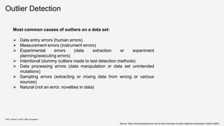
Data quality issues from regression task –
Missing values: refers when one variable or attribute does not contain any value. The missing values
occur when the source of data has a problem, e.g., sensor faults, faulty measurements, data transfer
problems or incomplete surveys.
Outlier: can be an observation univariate or multivariate. An observation is denominated an outlier
when it deviates markedly from other observations, in other words, when the observation appears to
be inconsistent respect to the remainder of observations.
High dimensionality: is referred to when dataset contains a large number of features. In this case, the
regression model tends to overfit, decreasing its performance.
Redundancy: represents duplicate instances in data sets which might detrimentally affect the
performance of classifiers.
Noise: defined as irrelevant or meaningless data. The data noisy reduce the predictive ability in a
regression model.](https://image.slidesharecdn.com/kdd2021tutorialfinal-210820164241/85/Data-Quality-for-Machine-Learning-Tasks-44-320.jpg)
![KDD Tutorial / © 2021 IBM Corporation
[DQR18]
Regression Task – Overview of Metrics
Data cleaning task from regression task –
Imputation: replaces missing data with substituted values. Four relevant approaches to imputing missing
values:
Deletion: excludes instances if any value is missing.
Hot deck: missing items are replaced by using values from the same dataset.
Imputation based on missing attribute: assigns a representative value to a missing one based on
measures of central tendency (e.g., mean, median, mode, trimmed mean).
Imputation based on non-missing attributes: missing attributes are treated as dependent variables, and a
regression or classification model is performed to impute missing values.
Outlier detection: identifies candidate outliers through approaches based on Clustering (e.g., DBSCAN:
Density-based spatial clustering of applications with noise) or Distance (e.g., LOF: Local Outlier Factor).](https://image.slidesharecdn.com/kdd2021tutorialfinal-210820164241/85/Data-Quality-for-Machine-Learning-Tasks-45-320.jpg)
![KDD Tutorial / © 2021 IBM Corporation
[DQR18]
Regression Task – Overview of Metrics
Data cleaning task from regression task –
Dimensionality reduction: reduces the number of attributes finding useful features to represent the dataset. A
subset of features is selected for the learning process of the regression model. The best subset of relevant
features is the one with least number of dimensions that most contribute to learning accuracy. Dimensionality
reduction can take on four approaches:
Filter: selects features based on discriminating criteria that are relatively independent of the regression
(e.g., correlation coefficients).
Wrapper: based on the performance of regression models (e.g., error measures) are maintained or
discarded features in each iteration.
Embedded: the features are selected when the regression model is trained. The embedded methods try to
reduce the computation time of the wrapper methods.
Projection: looks for a projection of the original space to space with orthogonal dimensions (e.g., principal
component analysis).
Remove duplicate instances: identifies and removes duplicate instances.](https://image.slidesharecdn.com/kdd2021tutorialfinal-210820164241/85/Data-Quality-for-Machine-Learning-Tasks-46-320.jpg)
![[DQR18]
Regression Task – Overview of Metrics](https://image.slidesharecdn.com/kdd2021tutorialfinal-210820164241/85/Data-Quality-for-Machine-Learning-Tasks-47-320.jpg)


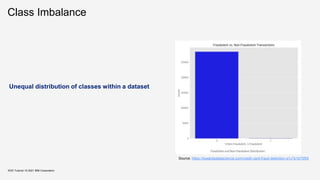
![Class Imbalance – for Regression
KDD Tutorial / © 2021 IBM Corporation
[SM13]
Several real-world prediction problems involve forecasting rare values of a target variable.
When this variable is nominal, we have a problem of class imbalance that was already studied
thoroughly within machine learning (classification task).
For regression tasks, where the target variable is continuous, few works exist addressing this type of
problem. Still, important application areas involve forecasting rare extreme values of a continuous target
variable.
Problem Statement
Predicting rare extreme values of a continuous variable is a
particular class of regression problems.
In this context, given a training sample of the problem, D = {hx, yi}N
i=1, our goal is to obtain a model that approximates the unknown
regression function y = f(x).
The particularity of our target tasks is that the goal is the predictive
accuracy on a particular subset of the domain of the target variable
Y - the rare and extreme values.](https://image.slidesharecdn.com/kdd2021tutorialfinal-210820164241/85/Data-Quality-for-Machine-Learning-Tasks-54-320.jpg)
![Class Imbalance – for Regression
KDD Tutorial / © 2021 IBM Corporation
[SM13]
Smote is a sampling method to address classification problems with imbalanced class distribution.
The key feature of this method is that it combines under-sampling of the frequent classes with over-
sampling of the minority class.
A variant of Smote for addressing regression tasks where the key goal is to accurately predict rare
extreme values, which we will name SmoteR.
There are three key components of the Smote algorithm that need to be address in order to adapt it for
our target regression tasks:
how to define which are the relevant observations and the ”normal” cases
how to create new synthetic examples (i.e. over-sampling)
how to decide the target variable value of these new synthetic examples](https://image.slidesharecdn.com/kdd2021tutorialfinal-210820164241/85/Data-Quality-for-Machine-Learning-Tasks-55-320.jpg)
![Class Imbalance – for Regression
KDD Tutorial / © 2021 IBM Corporation
[SM13]
There are three key components of the Smote algorithm that need to be address in order to adapt it for our
target regression tasks:
how to define which are the relevant observations and the ”normal” cases
original algorithm is based on the information provided by the user concerning which class value is
the target/rare class (usually known as the minority or positive class).
in regression problem, infinite number of values of the target variable are possible.
Solution - relevance function on a user-specified threshold on the relevance values, that leads to
the definition of the set Dr. Algorithm will over-sample the observations in Dr and under-sample the
remaining cases (Di), thus leading to a new training set with a more balanced distribution of the
values.](https://image.slidesharecdn.com/kdd2021tutorialfinal-210820164241/85/Data-Quality-for-Machine-Learning-Tasks-56-320.jpg)
![Class Imbalance – for Regression
KDD Tutorial / © 2021 IBM Corporation
[SM13]
how to create new synthetic examples (i.e. over-sampling)
Regards the second key component, the generation of new cases, same approach as in the original
SMOTE algorithm with some small modifications for being able to handle both numeric and nominal
attributes.](https://image.slidesharecdn.com/kdd2021tutorialfinal-210820164241/85/Data-Quality-for-Machine-Learning-Tasks-57-320.jpg)
![Class Imbalance – for Regression
KDD Tutorial / © 2021 IBM Corporation
[SM13]
how to decide the target variable value of these new synthetic examples
In the original algorithm this is a trivial question, because as all rare cases have the same class
(the target minority class), the same will happen to the examples generated from this set.
In our case the answer is not so trivial. The cases that are to be over-sampled do not have the
same target variable value, although they do have a high relevance score (φ(y)). This means that
when a pair of examples is used to generate a new synthetic case, they will not have the same
target variable value.
Proposed is to use a weighed average of the target variable values of the two seed examples. The
weights are calculated as an inverse function of the distance of the generated case to each of the
two seed examples.](https://image.slidesharecdn.com/kdd2021tutorialfinal-210820164241/85/Data-Quality-for-Machine-Learning-Tasks-58-320.jpg)

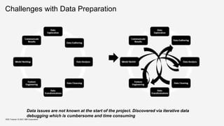
![Ordering/Sequence of data quality metrics to achieve better
performance
KDD Tutorial / © 2021 IBM Corporation
While there are several data quality issues that need to be addressed,
fixing these in an arbitrary order is shown to yield sub-optimal results.
as the search space of all possible sequences is combinatorically large, an important
challenge is to find the best sequence with respect to underlying task.
For example, authors in [FF12] suggest that correcting the data for missing values via missing
value imputation can affect outliers in the dataset.
This raises some interesting questions:
what should be the guiding factors by which such a sequence can be chosen,
how can we quantitatively measure these factors
is it possible to find an optimal sequence that allows us to maximize the ML classifier
performance](https://image.slidesharecdn.com/kdd2021tutorialfinal-210820164241/85/Data-Quality-for-Machine-Learning-Tasks-60-320.jpg)
![Ordering/Sequence of data quality metrics to achieve better
performance
KDD Tutorial / © 2021 IBM Corporation
Learn2Clean, a method based on Q-
Learning, a model-free reinforcement
learning technique
For a given dataset, it selects a ML model,
and a quality performance metric, the optimal
sequence of tasks for pre-processing the
data such that the quality of the ML model
result is maximized.
More intuitively, the problem that this work
address is the following: Given a dataset as
input D, a ML pipeline θ to apply to the input
dataset, a quality performance metric q, and
the space of all possible data preparation
and cleaning strategies Φ(D): Find the
dataset D ′ in Φ(D) that maximizes the quality
metric q
[FF12]](https://image.slidesharecdn.com/kdd2021tutorialfinal-210820164241/85/Data-Quality-for-Machine-Learning-Tasks-61-320.jpg)
![Ordering/Sequence of data quality metrics to
achieve better performance
KDD Tutorial / © 2021 IBM Corporation
[FF12]](https://image.slidesharecdn.com/kdd2021tutorialfinal-210820164241/85/Data-Quality-for-Machine-Learning-Tasks-62-320.jpg)

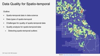
![Spatio-temporal data in data science
About 70% of tasks of ST data in data science
addresses prediction and detection by deep
learning models. [WCY20]
Example tasks:
Demand prediction
Flood forecast
KDD Tutorial / © 2021 IBM Corporation
spatial maps. ConvLSTM can be considered as a hybrid
del which combines RNN and CNN, and are usually used
handle spatial maps. AE and SDAE are mostly used to
n features from time series, trajectories and spatial maps.
2Seq model is generally designed for sequential data, and
s only used to handle time series and trajectories. The
rid models are also common for STDM. For example,
N and RNN can be stacked to learn the spatial features
, and then capture the temporal correlations among the
orical ST data. Hybrid models can be designed to fit all
four types of data representations. Other models such as
work embedding [164], multi-layer perceptron (MLP) [57],
6], generative adversarial nets (GAN) [49], [93], Residual
s [78], [89], deep reinforcement learning [50], etc. are also
d in recent works.
Addressing STDM Problems
inally, the selected or designed deep learning models are
d to address various STDM tasks such as classification,
dictivelearning, representation learning and anomaly detec-
. Note that usually how to select or design a deep learning
del depends on the particular data mining task and the input
a. However, to show the pipeline of the framework we first
way. Deep learning models are also used in other STDM
tasks including classification, detection, inference/estimation,
recommendation, etc. Next we will introduce the major STDM
problems in detail and summarize the corresponding deep
learning based solutions.
Fig. 14. Distributions of the STDM problems addressed by deep learning
models
Source S. Wang, J. Cao, and P. Yu, “Deep learning for spatio-temporal data mining: A survey,“ IEEE
Transactions on Knowledge and Data Engineering,2020.](https://image.slidesharecdn.com/kdd2021tutorialfinal-210820164241/85/Data-Quality-for-Machine-Learning-Tasks-68-320.jpg)
![Spatio-temporal data types
1. Event data
– Discrete events occurring at point locations and times. E.g., incidences of crime
events in the city
2. Trajectory data
– Paths traced by bodies moving in space over time. E.g., the patrol route of a
police surveillance car.
3. Point reference data
– Measurements of a continuous ST field such as temperature, vegetation, or
population over a set of moving reference points in space and time.
4. Raster data
– Measurements of a continuous or discrete ST field that are recorded at fixed
locations in space and at fixed time points. E.g., population density in geographic
information system)
KDD Tutorial / © 2021 IBM Corporation
[SJA15, WCY20]](https://image.slidesharecdn.com/kdd2021tutorialfinal-210820164241/85/Data-Quality-for-Machine-Learning-Tasks-69-320.jpg)
![Classical spatial outlier detection
- Local Moran’s I [Anselin95]
Spatial autocorrelation
Identify influential observations (e.g. hot spot, cold spot)
and outliers among the areas.
𝐼 =
𝑁
𝑊
𝑖 𝑗 𝑤𝑖𝑗
(𝑥𝑖
−𝑥)(𝑥𝑗
−𝑥)
𝑖 𝑥𝑖
−𝑥 2
where 𝑁 is the number of spatial units indexed by 𝑖 and 𝑗; 𝑥 is
the variable of interest; 𝑥 is the mean of 𝑥 ; 𝑤𝑖𝑗 is a matrix of
spatial weights with zeroes on the diagonal (i.e., 𝑤𝑖𝑗 = 0); and 𝑊
is the sum of all 𝑤𝑖𝑗.
KDD Tutorial / © 2021 IBM Corporation
3 2 0
5 8 1
2 4 1
(1) (2) (3)
(4) (5) (6)
(7) (8) (9)
Example
i,j = (1), (2), (3),...
xi = 3, 2, 0, ...
w12 = 1, w13 = 0, ...
1 2 3
1 1 2
2 1 3
Local Moran’s quadrant
Spatial values](https://image.slidesharecdn.com/kdd2021tutorialfinal-210820164241/85/Data-Quality-for-Machine-Learning-Tasks-72-320.jpg)
![Spatio-temporal Outlier Detection
“Spatio-temporal outlier detection is an extension of
spatial outlier detection.” [WLC10]
Spatio-temporal object is represented by a set of
instances 𝑜_𝑖𝑑, 𝑠𝑖, 𝑡𝑖 , where the spacestamp 𝑠𝑖, is
the location of object 𝑜_𝑖𝑑 at timestamp 𝑡𝑖.
Exact-Grid Top-K [WLC10] is a spatio-temporal outlier
detection algorithm that is based on:
Spatial Scan Statistic [Kulldorff97]
Exact-Grid [AMP06]
KDD Tutorial / © 2021 IBM Corporation
A moving region
Source:
[WLC10] E. Wu, W. Liu, and S. Chawla, “Spatio-temporal outlier detection in precipitation data,"
in Knowledge Discovery from Sensor Data, Springer Berlin Heidelberg, pp.115-133, 2010](https://image.slidesharecdn.com/kdd2021tutorialfinal-210820164241/85/Data-Quality-for-Machine-Learning-Tasks-74-320.jpg)
![Spatio-temporal Outlier Detection
- Spatial Scan Statistics [Kulldorff97]
Identify clusters of randomly positioned points
Determine hotspots in spatial data
Steps:
Study area observed events.
Place a point on the grid.
Observed and expected numbers of events are
recorded
Drawback: Huge amounts of calculation.
KDD Tutorial / © 2021 IBM Corporation
Source: Editing from https://rr-asia.oie.int/wp-content/uploads/2020/03/lecture-4_cluster-
detection-using-the-spatial-scan-statistic-satscan_20180920-min_vink.pdf](https://image.slidesharecdn.com/kdd2021tutorialfinal-210820164241/85/Data-Quality-for-Machine-Learning-Tasks-75-320.jpg)
![Spatio-temporal Outlier Detection
- Exact-Grid [AMP06]
A simple exact algorithm for finding the largest
discrepancy region in a domain.
Algorithm running in time 𝑂(𝑛4
) from 𝑂(𝑛5
)
Approximation algorithm for a large class of
discrepancy functions (including the Kulldorff scan
statistic).
KDD Tutorial / © 2021 IBM Corporation
Figure 1: Exam ple of m axim al discrepancy range
on a dat a set . X s are m easur ed dat a and Os are
baseline dat a.
An equi
point r =
Pr obl e
ancy func
range R ∈
In this p
ing of axis
the same s
crepancy
axis-parall
B oundar
fitting, we
very small
Formally,
has a mea
C ≥ 1.
equivalent
Sn = [C/
care about
than base
{ (mR , bR )
Example of maximal discrepancy range on a data set.
pr
pl
pb
(a) Sweep Line in Algo-
rithm Exact .
r
r∗
Cr ∗
Cr
p
q
ui = nr
(b) Error between contours.
φ
φ
2
<
l
2
h
φ
(c) Error in approximating
an arc with a segment.
Figure 2: Sweep lines, cont ours, and arcs.
Grid algorit hm s. For some algorithms, the data is as-
sumed to lie on a grid, or is accumulated onto a set of
A lgor it hm 1 Algorithm Exact
maxd = -1
Techniques that the algorithm uses
[AMP06] Deepak Agarwal, Andrew McGregor, Jeff M Philipps, et al. "Spatial scan statistics: approximations and performance
study." Proceedings of the 12th ACM SIGKDD international conference on Knowledge discovery and data mining. 2006.](https://image.slidesharecdn.com/kdd2021tutorialfinal-210820164241/85/Data-Quality-for-Machine-Learning-Tasks-76-320.jpg)
![Spatio-temporal Outlier Detection
- Exact-Grid Top-k [WLC10]
Extend Exact-Grid and Approx-Grid algorithms for
overlapping problem. Find the top-k outliers in a spatial
grid for each time period.
Finding the top-k outliers
Find every possible region size and shape in the grid.
Get each region’s discrepancy value to determine
which is a more significant outlier.
Keeps track of the top-k regions rather than just the
top-1.
KDD Tutorial / © 2021 IBM Corporation
left right
top
bottom
Overlap problem
Finding Top-k algorithm
Source: https://slideplayer.com/slide/4806555/
[WLC10] E. Wu, W. Liu, and S. Chawla, “Spatio-temporal outlier detection in precipitation data,"
in Knowledge Discovery from Sensor Data, Springer Berlin Heidelberg, pp.115-133, 2010](https://image.slidesharecdn.com/kdd2021tutorialfinal-210820164241/85/Data-Quality-for-Machine-Learning-Tasks-77-320.jpg)
![Summary of Data Quality for Spatio-temporal
Spatio-temporal data in data science
Retail sales analysis, Transportation
Data types of spatio-temopral
Event ,trajectory point reference, and raster data
Challenges for quality of spatio-temporal data
Outlier of ST data
Quality analysis for spatio-temporal data
Spatial Scan Statistics [Kulldorff97], Exact-Grid [AMP06, WLC10]
KDD Tutorial / © 2021 IBM Corporation](https://image.slidesharecdn.com/kdd2021tutorialfinal-210820164241/85/Data-Quality-for-Machine-Learning-Tasks-78-320.jpg)


![Dataset Cartography:
Mapping and Diagnosing Datasets with Training Dynamics
Objective:
Leverage the behavior of the ML model on individual instances during training to generate a data map
that illustrates easy-to-learn, hard-to-learn and ambiguous samples in the dataset.
Approach:
1. Measure the confidence, correctness and variability of the model during training epochs.
2. Model confidence is measured as the mean probability of the true label across training epochs.
3. Model correctness is measured as the fraction of times the model correctly predicts the label.
4. Model variability is measured as the standard deviation of the predicted probabilities of the true
label across training epochs.
Task:
Compare performance of various baselines generated by selecting subsets of the dataset and training
the RoBERTA large model.
KDD Tutorial / © 2021 IBM Corporation
Source : Swayamdipta, Swabha, et al. 2020, Dataset Cartography: Mapping and Diagnosing Datasets with Training Dynamics
[SSL+20]](https://image.slidesharecdn.com/kdd2021tutorialfinal-210820164241/85/Data-Quality-for-Machine-Learning-Tasks-86-320.jpg)
![KDD Tutorial / © 2021 IBM Corporation
Source : Swayamdipta, Swabha, et al. 2020, Dataset Cartography: Mapping and Diagnosing Datasets with Training Dynamics
Dataset Cartography:
Mapping and Diagnosing Datasets with Training Dynamics
Data Map and Insights:
Data follows a bell-shaped curve with respect to
confidence and variability
correctness determines discrete regions
Instances with high confidence and low variability
region of the map (top-left) are easy-to-learn
Instances with low variability and low confidence
(bottom-left) are hard-to-learn
Instances with high variability (right) are ambiguous
hard-to-learn and ambiguous instances are most
informative for learning.
Some amount of easy-to-learn instances are also
necessary for successful optimization
[SSL+20]](https://image.slidesharecdn.com/kdd2021tutorialfinal-210820164241/85/Data-Quality-for-Machine-Learning-Tasks-87-320.jpg)
![Data Valuation Using Reinforcement Learning
Objective:
Determine a reward for each sample by quantifying the performance of the predictor model on a small validation
set and use it as a reinforcement signal to learn the likelihood of the sample being using in training of the
predictor model.
Approach:
1. Perform end-to-end training of (i) target task predictor model and (ii) data value estimator model
2. Data value estimator generates selection probabilities for a mini-batch of training samples
3. Predictor model trains on the mini-batch and loss is computed against the validation set
4. Predictor model parameters are updated through back-propagation
5. Data value estimator parameters are updated using the Reinforce approach
Task:
1. Compare DVRL framework against standard baselines on standard datasets from different domains
KDD Tutorial / © 2021 IBM Corporation
Source : Yoon, Jinsung et. al 2020, Data valuation using reinforcement learning
[YAP20]](https://image.slidesharecdn.com/kdd2021tutorialfinal-210820164241/85/Data-Quality-for-Machine-Learning-Tasks-88-320.jpg)
![Data Valuation Using Reinforcement Learning
KDD Tutorial / © 2021 IBM Corporation
Insights:
Using only 60%-70% of the training set (the highest valued samples), DVRL can obtain a similar performance compared to training
on the entire dataset.
The framework also outperforms baselines in the presence of noisy labels and is able to detect noisy labels in the dataset by
assigning them low scores.
The computational complexity of DVRL framework, instead of being exponential in terms of the dataset size, the overhead is only
twice of conventional training.
Source : Yoon, Jinsung et. al 2020, Data valuation using reinforcement learning
[YAP20]](https://image.slidesharecdn.com/kdd2021tutorialfinal-210820164241/85/Data-Quality-for-Machine-Learning-Tasks-89-320.jpg)

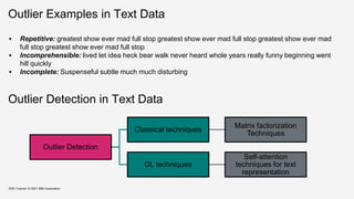
![Outlier Detection for Text Data
Feature Generation – Simple Bag of Words
Approach
Apply Matrix Factorization – Decompose the
given term matrix into a low rank matrix L and
an outlier matrix Z
Further, L can be expressed as
where,
The l2 norm score of a particular column zx
serves as an outlier score for the document
KDD Tutorial / © 2021 IBM Corporation
Source : Kannan et al, 2017. Outlier detection for text data
[KWAP17]](https://image.slidesharecdn.com/kdd2021tutorialfinal-210820164241/85/Data-Quality-for-Machine-Learning-Tasks-93-320.jpg)
![Outlier Detection for Text Data
For experiments, outliers are sampled from a unique class from standard datasets
Receiver operator characteristics are studied to assess the performance of the
proposed approach.
Approach is useful at identifying outliers even from regular classes.
Patterns such as unusually short/long documents, unique words, repetitive vocabulary
etc. were observed in detected outliers.
KDD Tutorial / © 2021 IBM Corporation
Source : Kannan et al, 2017. Outlier detection for text data
[KWAP17]](https://image.slidesharecdn.com/kdd2021tutorialfinal-210820164241/85/Data-Quality-for-Machine-Learning-Tasks-94-320.jpg)
![Unsupervised Anomaly Detection on Text
Multi-Head Self-Attention:
KDD Tutorial / © 2021 IBM Corporation
Sentence Embedding
Attention matrix
Proposes a novel one-class classification method which leverages pretrained word
embeddings to perform anomaly detection on text
Given a word embedding matrix H, multi-head self-attention is used to map sentences of
variable length to a collection of fixed size representations, representing a sentence with
respect to multiple contexts
Source : Ruff et al 2019. Self-Attentive, Multi-Context One-Class Classification for Unsupervised Anomaly Detection on Text
(1)
(2)
[RZV+19]](https://image.slidesharecdn.com/kdd2021tutorialfinal-210820164241/85/Data-Quality-for-Machine-Learning-Tasks-95-320.jpg)
![Unsupervised Anomaly Detection on Text
KDD Tutorial / © 2021 IBM Corporation
CVDD Objective
Context Vector
Orthogonality Constraint
These sentence representations are trained along with a collection of context vectors such that
the context vectors and representations are similar while keeping the context vectors diverse
Greater the distance of mk(H) to ck implies a more anomalous sample w.r.t. context k
Outlier Scoring
(1)
Source : Ruff et al 2019. Self-Attentive, Multi-Context One-Class Classification for Unsupervised Anomaly Detection on Text
[RZV+19]](https://image.slidesharecdn.com/kdd2021tutorialfinal-210820164241/85/Data-Quality-for-Machine-Learning-Tasks-96-320.jpg)

![EDA: Easy Data Augmentation Techniques for Boosting
Performance on Text Classification Tasks
Objective:
Utilize simple text operators to perform data augmentation and boost performance of ML models on text
classification tasks specifically for small datasets.
Approach:
1. Four specific text operators are discussed – (i) synonym replacement (ii) random insertion (iii) random
swap and (iv) random deletion
2. For a given sentence in the training set, one of the operations is performed at random.
3. The number of words changed, n, is based on the sentence length l with the formula n=αl.
4. For each original sentence, naug augmented sentences are generated.
Task:
1. Compare EDA on five NLP tasks with CNNs and RNNs
KDD Tutorial / © 2021 IBM Corporation
Wei, Jason, and Kai Zou, 2019, Eda: Easy data augmentation techniques for boosting performance on text classification tasks.
[WZ19]](https://image.slidesharecdn.com/kdd2021tutorialfinal-210820164241/85/Data-Quality-for-Machine-Learning-Tasks-98-320.jpg)
![EDA: Easy Data Augmentation Techniques for Boosting
Performance on Text Classification Tasks
KDD Tutorial / © 2021 IBM Corporation
Insights:
Average improvement of 0.8% for full datasets
and 3.0% for Ntrain=500 is observed
For the training set fractions {1, 5, 10, 20, 30, 40}
there is consistent and significant improvement
observed across all datasets and tasks
It is empirically shown that EDA conserves the
labels the original sentence by analyzing t-SNE
plots of augmented samples
Some of the limitations are (i) performance gain
can be marginal when data is sufficient and (ii)
EDA might not yield substantial improvements
when using pre-trained models
Wei, Jason, and Kai Zou, 2019, Eda: Easy data augmentation techniques for boosting performance on text classification tasks.
[WZ19]](https://image.slidesharecdn.com/kdd2021tutorialfinal-210820164241/85/Data-Quality-for-Machine-Learning-Tasks-99-320.jpg)
![Do not Have Enough Data? Deep Learning to the
Rescue!
Objective:
Given a small labelled dataset, perform data augmentation by generating synthetic samples using a pre-trained
language model fine-tuned on the dataset.
Approach:
1. Use a pre-trained language model (GPT-2) to fine-tune on the available labelled dataset and use it to
synthesize new labelled sentences.
2. Independently, train a classifier on the original dataset and use it to filter the synthesized data corpus by
filtering out synthesized samples with low classifier confidence score.
Task:
1. Compare LAMBADA framework against SOA baselines on standard datasets to compare performance.
KDD Tutorial / © 2021 IBM Corporation
Source : Anaby-Tavor, Ateret, et al., 2020, Do not have enough data? Deep learning to the rescue!.
[ATCG+20]](https://image.slidesharecdn.com/kdd2021tutorialfinal-210820164241/85/Data-Quality-for-Machine-Learning-Tasks-100-320.jpg)
![Do not Have Enough Data? Deep Learning to the
Rescue!
KDD Tutorial / © 2021 IBM Corporation
Insights:
Proposed framework is compared against various
classifier models against different baselines on 3
standard datasets.
It is empirically shown that LAMBADA approach shows
improvement in performance with upto 50 samples per
class and it is classifier agnostic.
When compared with SOA baselines, LAMBADA
consistently performs better on all the datasets with
various classifiers.
Experiments are also done to show that LAMBADA can
also serve as an alternative to semi-supervised
techniques when unlabelled data does not exist.
Source : Anaby-Tavor, Ateret, et al., 2020, Do not have enough data? Deep learning to the rescue!.
[ATCG+20]](https://image.slidesharecdn.com/kdd2021tutorialfinal-210820164241/85/Data-Quality-for-Machine-Learning-Tasks-101-320.jpg)

![Evolutionary Data Measures: Understanding the Difficulty
of Text Classification Tasks
Proposes an approach to design data quality metric which
explains the complexity of the given data for classification task
Considers various data characteristics to generates a 48 dim
feature vector for each dataset.
Data characteristics include
Class Diversity: Count based probability distribution of classes in
the dataset
Class Imbalance: 𝑐=1
𝐶
|
1
𝐶
−
𝑛𝑐
𝑇𝑑𝑎𝑡𝑎
|
Class Interference: Similarities among samples belonging to
different classes
Data Complexity: Linguistic properties of data samples
KDD Tutorial / © 2021 IBM Corporation
Source : Collins et al, 2018. Evolutionary Data Measures: Understanding the Difficulty of Text Classification Tasks
Feature vector for a given dataset cover
quality properties such as
Class Diversity (2-Dim)
Shannon Class Diversity
Shannon Class Equitability
Class Imbalance (1-Dim)
Class Interference (24-Dim)
Hellinger Similarity
Top N-Gram Interference
Mutual Information
Data Complexity (21-Dim)
Distinct n-gram : Total n-gram
Inverse Flesch Reading Ease
N-Gram and Character diversity
[CRZ18]](https://image.slidesharecdn.com/kdd2021tutorialfinal-210820164241/85/Data-Quality-for-Machine-Learning-Tasks-103-320.jpg)
![Understanding the Difficulty of Text Classification Tasks
Authors propose usage of genetic algorithms to intelligently explore the 248 possible combinations
The fitness function for the genetic algorithm was Pearson correlation between difficulty score and
model performance on test set
89 datasets were considered for evaluation and 12 different types of models on each dataset
The effectiveness of a given combination of metric is measured using its correlation with the
performance of various models on various datasets
Stronger the negative correlation of a metric with model performance, better the metric explains data
complexity
KDD Tutorial / © 2021 IBM Corporation
Source : Collins et al, 2018. Evolutionary Data Measures: Understanding the Difficulty of Text Classification Tasks
[CRZ18]](https://image.slidesharecdn.com/kdd2021tutorialfinal-210820164241/85/Data-Quality-for-Machine-Learning-Tasks-104-320.jpg)
![Understanding the Difficulty of Text Classification Tasks
KDD Tutorial / © 2021 IBM Corporation
Difficulty Measure D2 =
Distinct Unigrams : Total Unigrams + Class Imbalance +
Class Diversity + Maximum Unigram Hellinger Similarity
+ Unigram Mutual Info.
Correlation = −0.8814
Source : Collins et al, 2018. Evolutionary Data Measures: Understanding the Difficulty of Text Classification Tasks
[CRZ18]](https://image.slidesharecdn.com/kdd2021tutorialfinal-210820164241/85/Data-Quality-for-Machine-Learning-Tasks-105-320.jpg)


![References
KDD Tutorial / © 2021 IBM Corporation
[BF99] Carla E Brodley and Mark A Friedl. Identifying mislabeled training data. Journal of artificial intelligence research, 11:131–167, 1999.
[ARK18] Mohammed Al-Rawi and Dimosthenis Karatzas. On the labeling correctness in computer vision datasets. In IAL@PKDD/ECML, 2018.
[NJC19] Curtis G Northcutt, Lu Jiang, and Isaac L Chuang. Confident learning: Estimating uncertainty in dataset labels. arXiv preprint
arXiv:1911.00068, 2019.
[EGH17] Rajmadhan Ekambaram, Dmitry B Goldgof, and Lawrence O Hall. Finding label noise examples in large scale datasets. In2017 IEEE
International Conference on Systems, Man, and Cybernetics pages 2420–2424., 2017.
[XHJ10] Xiong, Haitao, Junjie Wu, and Lu Liu. "Classification with class overlapping: A systematic study." The 2010 International Conference on
E-Business Intelligence. 2010
[DQT21] Nitin Gupta, Hima Patel, Shazia Afzal, Naveen Panwar, Ruhi Sharma Mittal, Shanmukha Guttula, Abhinav Jain, Lokesh Nagalapatti,
Sameep Mehta, Sandeep Hans, Pranay Lohia, Aniya Aggarwal, Diptikalyan Saha. Data Quality Toolkit: Automatic assessment of data quality
and remediation for machine learning datasets. arXiv, 2021, https://arxiv.org/pdf/2108.05935.pdf
[FF12] W. Fan and F. Geerts, “Foundations of data quality management,”Syn-thesis Lectures on Data Management, vol. 4, no. 5, pp. 1–217,
2012
[DQR18] Corrales, David Camilo, Juan Carlos Corrales, and Agapito Ledezma. "How to address the data quality issues in regression models: a
guided process for data cleaning." Symmetry 10.4 (2018): 99.](https://image.slidesharecdn.com/kdd2021tutorialfinal-210820164241/85/Data-Quality-for-Machine-Learning-Tasks-109-320.jpg)
![References
KDD Tutorial / © 2021 IBM Corporation
[OT21] Agarwal, Amulya, and Nitin Gupta. "Comparison of Outlier Detection Techniques for Structured Data." arXiv preprint
arXiv:2106.08779 (2021).
[SM13] Torgo, Luís, et al. "Smote for regression." Portuguese conference on artificial intelligence. Springer, Berlin, Heidelberg, 2013.
WCY20] S. Wang, J. Cao, and P. Yu, “Deep learning for spatio-temporal data mining: A survey," IEEE Transactions on Knowledge and Data
Engineering,2020.
[SJA15] S. Shekhar, Z. Jiang, R. Y. Ali, et al., “Spatiotemporal data mining: A computational perspective,” ISPRS International Journal of Geo-
Information, vol. 4, no. 4, pp. 2306-2338, 2015.
[WLC10] E. Wu, W. Liu, and S. Chawla, “Spatio-temporal outlier detection in precipitation data," in Knowledge Discovery from Sensor Data,
Springer Berlin Heidelberg, pp.115-133, 2010
[GGA14] M. Gupta, J. Gao, C. C. Aggarwal, and J. Han, “Outlier detection for temporal data: A survey," IEEE Transactions on Knowledge and
Data Engineering, vol. 26, no. 9, pp. 2250-2267, 2014.
[KN98] E. M. Knorr and R. T. Ng, “Algorithms for mining distance-based outliers in large datasets," in Proceedings of the 24th International
Conference on Very Large Data Bases, ser. VLDB '98. San Francisco, CA, USA: Morgan Kaufmann Publishers Inc., 1998, p. 392-403.](https://image.slidesharecdn.com/kdd2021tutorialfinal-210820164241/85/Data-Quality-for-Machine-Learning-Tasks-110-320.jpg)
![References
KDD Tutorial / © 2021 IBM Corporation
[SLZ01] S. Shekhar, C.-T. Lu, and P. Zhang, “Detecting graph-based spatial outliers: Algorithms and applications (a summary of results)," in
Proceedings of the Seventh ACM SIGKDD International Conference on Knowledge Discovery and Data Mining, ser. KDD '01. New York, NY,
USA: Association for Computing Machinery, 2001, p. 371-376.
[CL04] T. Cheng and Z. Li, “A hybrid approach to detect spatio-temporal outliers," in Proceedings of the 12th International Conference on
Geoinformatics, 2004, p. 173-178
[Anselin95] Anselin, Luc. "Local indicators of spatial association—LISA." Geographical analysis 27.2 (1995): 93-115.
[AMP06] Deepak Agarwal, Andrew McGregor, Jeff M Philipps, et al. "Spatial scan statistics: approximations and performance
study." Proceedings of the 12th ACM SIGKDD international conference on Knowledge discovery and data mining. 2006.
[SSL+20] Swabha Swayamdipta, Roy Schwartz, Nicholas Lourie, Yizhong Wang, Hannaneh Hajishirzi, Noah A Smith, and Yejin Choi. Dataset
cartography: Mapping and diagnosing datasets with training dynamics. In Proceedings of the 2020 Conference on Empirical Methods in Natural
Language Processing (EMNLP), pages 9275–9293, 2020.
[WZ19] Jason Wei and Kai Zou. Eda: Easy data augmentation techniques for boosting performance on text classification tasks. In Proceedings of
the 2019 Conference on Empirical Methods in Natural Language Processing and the 9th International Joint Conference on Natural Language
Processing (EMNLP-IJCNLP), pages 6382–6388, 2019.](https://image.slidesharecdn.com/kdd2021tutorialfinal-210820164241/85/Data-Quality-for-Machine-Learning-Tasks-111-320.jpg)
![References
KDD Tutorial / © 2021 IBM Corporation
[ATCG+20] Ateret Anaby-Tavor, Boaz Carmeli, Esther Goldbraich, Amir Kantor, George Kour, Segev Shlomov, Naama Tepper, and Naama
Zwerdling. Do not have enough data? Deep learning to the rescue! In Proceedings of the AAAI Conference on Artificial Intelligence, volume
34, pages 7383–7390, 2020.
[CRZ18] Edward Collins, Nikolai Rozanov, and Bingbing Zhang. Evolutionary data measures: Understanding the difficulty of text classification
tasks. arXiv preprintarXiv:1811.01910, 2018.
[KWAP17] Ramakrishnan Kannan, Hyenkyun Woo, Charu C Aggarwal, and Haesun Park. Outlier detection for text data. In Proceedings of the
2017 siam international conference ondata mining, pages 489–497. SIAM, 2017.
[RWGS20] Marco Tulio Ribeiro, Tongshuang Wu, Carlos Guestrin, and Sameer Singh. Beyond accuracy: Behavioral testing of nlp models
with checklist.arXiv preprintarXiv:2005.04118, 2020.
[RZV+19] Lukas Ruff, Yury Zemlyanskiy, Robert Vandermeulen, Thomas Schnake, and Marius Kloft. Self-attentive, multi-context one-class
classification for unsupervised anomaly detection on text. In Proceedings of the 57th Annual Meeting of the Association for Computational
Linguistics, pages 4061–4071, 2019.
[YAP20] Jinsung Yoon, Sercan Arik, and Tomas Pfister. Data valuation using reinforcement learning. InInternational Conference on Machine
Learning, pages 10842–10851. PMLR,2020.](https://image.slidesharecdn.com/kdd2021tutorialfinal-210820164241/85/Data-Quality-for-Machine-Learning-Tasks-112-320.jpg)

The document outlines the importance of data quality in machine learning, emphasizing that data preparation is a time-consuming and critical aspect of the AI development lifecycle. It highlights the need for automated data quality analysis tools and introduces the concept of 'data quality 2.0', which shifts focus to metrics suited for assessing data in the context of machine learning models. Additionally, it discusses various data quality metrics, challenges in managing different data modalities, and emphasizes the crucial relationship between data quality and the effectiveness of machine learning algorithms.


![ViT (Vision Transformer) Review [CDM]](https://cdn.slidesharecdn.com/ss_thumbnails/vitreviewcdm-201012184226-thumbnail.jpg?width=640&height=640&fit=bounds)


![[系列活動] 資料探勘速遊](https://cdn.slidesharecdn.com/ss_thumbnails/0114ycchendmquicktour-170110050658-thumbnail.jpg?width=640&height=640&fit=bounds)


