Downloaded 11 times


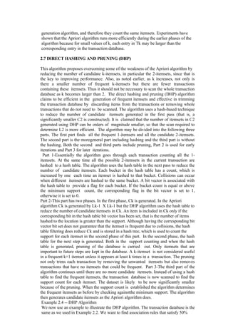


![4.6 PARTITIONAL METHODS
Partitional methods are popular since they tend to be computationally efficient and are
more easily adapted for very large datasets.
The K-Means Method
K-Means is the simplest and most popular classical clustering method that is easy
toimplement. The classical method can only be used if the data about all the objects
islocated in the main memory. The method is called K-Means since each of the K clusters
is represented by the mean of the objects (called the centroid) within it. It is also called
the centroid method since at each step the centroid point of each cluster is assumed to be
known and each of the remaining points are allocated to the cluster whose centroid is
closest to it.
he K-means method uses the Euclidean distance measure, which appears towork well
with compact clusters. The K-means method may be described as follows:
1. Select the number of clusters. Let this number be k.
2. Pick k seeds as centroids of the k clusters. The seeds may be picked randomly unless
the user has some insight into the data.
3. Compute the Euclidean distance of each object in the dataset from each of the
centroids.
4. Allocate each object to the cluster it is nearest to based on the distances computed in
the previous step.
5. Compute the centroids of the clusters by computing the means of the
attribute values of the objects in each cluster.
6. Check if the stopping criterion has been met (e.g. the cluster membership
is unchanged). If yes, go to Step 7. If not, go to Step 3.7. [Optional] One may decide
tostop at this stage or to split a cluster or combine two clusters heuristically until a
stopping criterion is met. The method is scalable and efficient (the time complexity is of
O(n)) and is guaranteed to find a local minimum.
4.7 HIERARCHICAL METHODS
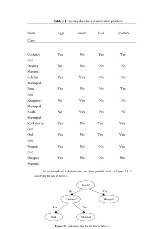
Hierarchical methods produce a nested series of clusters as opposed to the partitional](https://image.slidesharecdn.com/fjkrziqusgsfkciwlwfe-140620121355-phpapp01/85/ii-mca-juno-33-320.jpg)


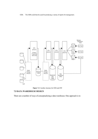


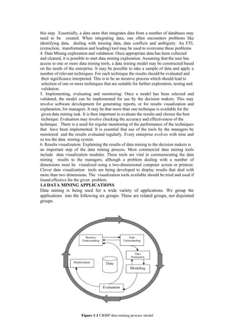
Data mining involves using analytical techniques to discover patterns in large data sets. It is used to gain insights into business problems like predicting customer behavior or identifying fraud. The key steps in data mining include requirement analysis, data collection/preparation, exploration of techniques, implementation/evaluation, and visualization of results. Applications include prediction, relationship marketing, customer profiling, outlier detection, and customer segmentation.