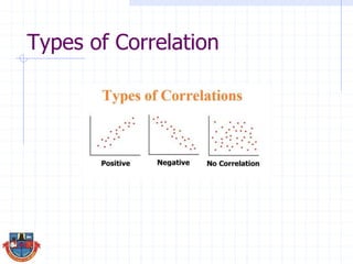
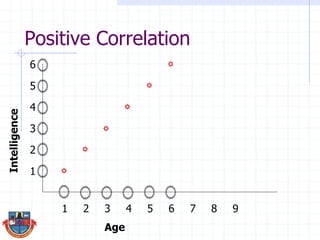
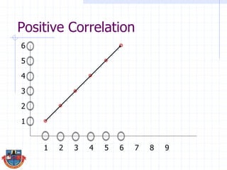
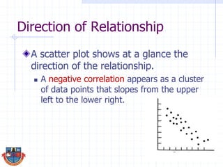
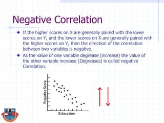
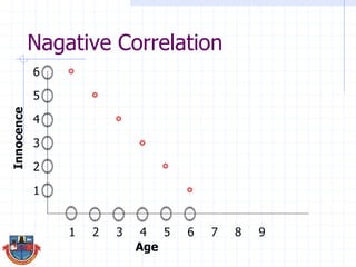
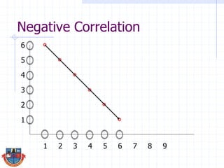
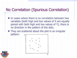
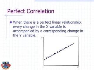
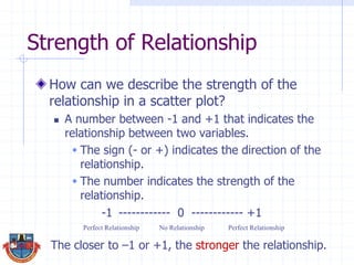
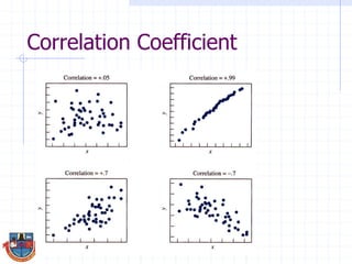
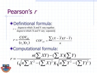
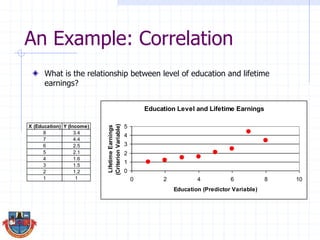
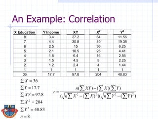
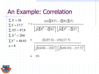
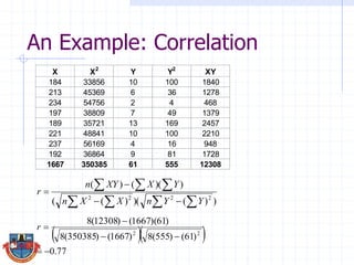
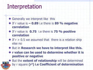
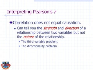
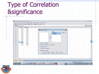
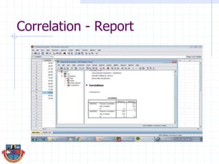
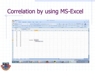
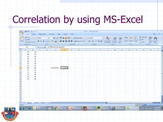
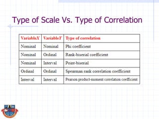
The document discusses correlation and how it is used to measure the strength and direction of relationships between two variables. Correlation coefficients range from -1 to 1, where -1 is a perfect negative correlation, 0 is no correlation, and 1 is a perfect positive correlation. The document provides examples of calculating correlation coefficients using Pearson's r formula and interpreting the results, demonstrating both positive and negative correlations between variables like education level and lifetime earnings.

1. Correlation
Correlation is a statistical technique which can
show whether and how strongly pairs of variables
are related. For example, height and weight are
related - taller people tend to be heavier than
shorter people.

2. Correlation
Correlation is used to measure and
describe a relationship between two
variables.
Usually these two variables are simply
observed as they exist in the
environment; there is no attempt to
control or manipulate the variables.

3. Correlation
The correlation coefficient measures
two characteristics of the relationship
between X and Y:
 The direction of the relationship.
 The degree of the relationship.
Product Moment Correlation was developed
by Karl Pearson. (Pearson’s r)

4. Types of Correlation

5. Direction of Relationship
A scatter plot shows at a glance the
direction of the relationship.
 A positive correlation appears as a cluster
of data points that slopes from the lower
left to the upper right.

6. Positive Correlation
If the higher scores on X are generally paired with the higher
scores on Y, and the lower scores on X are generally paired with
the lower scores on Y, then the direction of the correlation
between two variables is positive.
As the value of one variable increases (Degreases) the value of
the other variable increase (Degreases) is called passitive
Correlation.

7. Positive Correlation
1 2 3 4 5 6 7 8 9
1
2
3
4
5
6
Age
Intelligence

8. Positive Correlation
1 2 3 4 5 6 7 8 9
1
2
3
4
5
6

9. Direction of Relationship
A scatter plot shows at a glance the
direction of the relationship.
 A negative correlation appears as a cluster
of data points that slopes from the upper
left to the lower right.

10. Negative Correlation
If the higher scores on X are generally paired with the lower
scores on Y, and the lower scores on X are generally paired with
the higher scores on Y, then the direction of the correlation
between two variables is negative.
As the value of one variable degrease (increase) the value of
the other variable increase (Degreases) is called negative
Correlation.

11. Nagative Correlation
1 2 3 4 5 6 7 8 9
1
2
3
4
5
6
Age
Innocence

12. Negative Correlation
1 2 3 4 5 6 7 8 9
1
2
3
4
5
6

13. No Correlation (Spurious Correlation)
In cases where there is no correlation between two
variables (both high and low values of X are equally
paired with both high and low values of Y), there is
no direction in the pattern of the dots.
They are scattered about the plot in an irregular
pattern.

14. Perfect Correlation
When there is a perfect linear relationship,
every change in the X variable is
accompanied by a corresponding change in
the Y variable.

15. Form of Relationship
Pearson’s r assumes an underlying
linear relationship (a relationship that
can be best represented by a straight
line).
Not all relationships are linear.

16. Strength of Relationship
How can we describe the strength of the
relationship in a scatter plot?
 A number between -1 and +1 that indicates the
relationship between two variables.
 The sign (- or +) indicates the direction of the
relationship.
 The number indicates the strength of the
relationship.
-1 ------------ 0 ------------ +1
Perfect Relationship No Relationship Perfect Relationship
The closer to –1 or +1, the stronger the relationship.

17. Correlation Coefficient

18. Pearson’s r
Definitional formula:
))()()((
))(()(
2222





YYnXXn
YXXYn
r
r 
COVXY
(sx )(sy) n
YYXX
COVXY
 

))((
separatelyvaryYandXwhichtodegree
thervary togeYandXwhichtodegree
r
Computational formula:

19. An Example: Correlation
What is the relationship between level of education and lifetime
earnings?
Education Level and Lifetime Earnings
0
1
2
3
4
5
0 2 4 6 8 10
Education (Predictor Variable)
LifetimeEarnings
(CriterionVariable)
X (Education) Y (Income)
8 3.4
7 4.4
6 2.5
5 2.1
4 1.6
3 1.5
2 1.2
1 1

20. An Example: Correlation
X Education Y Income XY X2
Y2
8 3.4 27.2 64 11.56
7 4.4 30.8 49 19.36
6 2.5 15 36 6.25
5 2.1 10.5 25 4.41
4 1.6 6.4 16 2.56
3 1.5 4.5 9 2.25
2 1.2 2.4 4 1.44
1 1 1 1 1
36 17.7 97.8 204 48.83
8
83.48
204
8.97
7.17
36
2
2






n
Y
X
XY
Y
X
))()()((
))(()(
2222





YYnXXn
YXXYn
r

21. An Example: Correlation
8
83.48
204
8.97
7.17
36
2
2






n
Y
X
XY
Y
X

22. An Example: Correlation
))()()((
))(()(
2222





YYnXXn
YXXYn
r
X X2
Y Y2
XY
184 33856 10 100 1840
213 45369 6 36 1278
234 54756 2 4 468
197 38809 7 49 1379
189 35721 13 169 2457
221 48841 10 100 2210
237 56169 4 16 948
192 36864 9 81 1728
1667 350385 61 555 12308
  
77.0
)61()555(8)1667()350385(8
)61)(1667()12308(8
22



r

23. Interpretation
Generally we interpret like this
If r value is – 0.89 i.e there is 89 % negative
correlation
If r value is 0.75 i.e there is 75 % positive
correlation
If r > 0.5 we assumed that there is a relation ship
else no
But in Research we have to interpret like this.
r value can be used to determine whether it is
positive or negative
But the extent of relationship will be determined
by r square (r2) i.e Coefficient of determination

24. Interpreting Pearson’s r
Correlation does not equal causation.
 Can tell you the strength and direction of a
relationship between two variables but not
the nature of the relationship.
 The third variable problem.
 The directionality problem.

25. Running Correlation by SPSS

26. Running Correlation by SPSS

27. Type of Correlation
&significance

28. Correlation - Report

29. Correlation by using MS-Excel

30. Correlation by using MS-Excel

31. Correlation by LibreOffice

32. Type of Scale Vs. Type of Correlation