The document discusses a new algorithm for computing the Wiener index of Fibonacci weighted trees with Fibonacci branching, reducing the computational complexity to logarithmic time. The Wiener index is important in graph theory and has applications in mathematical chemistry, serving as a distance-based invariant that correlates with organic compound properties. The research provides insights into calculating distances between vertex pairs in edge-weighted graphs more efficiently than using traditional methods.
![Natarajan Meghanathan, et al. (Eds): SIPM, FCST, ITCA, WSE, ACSIT, CS & IT 06, pp. 471–478, 2012.
© CS & IT-CSCP 2012 DOI : 10.5121/csit.2012.2346
COMPUTING WIENER INDEX OF FIBONACCI
WEIGHTED TREES
K. R. Udaya Kumar Reddy1
and Ranjana S. Chakrasali2
1, 2
Department of Computer Science and Engineering, BNM Institute of
Technology, Bangalore-560070, Karnataka, India
{krudaykumar@yahoo.com, ranjanagirish@gmail.com}
ABSTRACT
Given a simple connected undirected graph ܩ = ሺܸ, ܧሻ with |ܸ| = ݊ and ||ܧ = ݉, the Wiener
index ܹሺܩሻ of ܩ is defined as half the sum of the distances of the form ݀ሺ,ݑ ݒሻ between all
pairs of vertices u, v of ܩ . If ሺ,ܩ ݓாሻ is an edge-weighted graph, then the Wiener
index ܹሺ,ܩ ݓாሻof ሺ,ܩ ݓாሻ is defined as the usual Wiener index but the distances is now
computed in ሺ,ܩ ݓாሻ. The paper proposes a new algorithm for computing the Wiener index of a
Fibonacci weighted trees with Fibonacci branching in place of the available naive algorithm for
the same. It is found that the time complexity of the algorithm is logarithmic.
KEYWORDS
Algorithms, Distance in graphs, Fibonacci weighted tree, Wiener index.
1. INTRODUCTION
Let ܩ = ሺܸሺܩሻ, ܧሺܩሻሻ be a connected unweighted undirected graph without self-loops and
multiple edges. Let |ܸሺܩሻ| = ݊ and |ܧሺܩሻ| = ݉.
The Wiener index ܹሺܩሻ of ܩ is defined as half the sum of the distances between all pairs of
vertices of a graph .ܩ Wiener index is a distance based graph invariant which is one of the most
popular topological indices in mathematical chemistry. It is named after the chemist Harold
Wiener, who first introduced it in 1947 to study chemical properties of alkanes. It is not
recognized that there are good correlations between ܹሺܩሻ and physico-chemical properties of the
organic compound from which ܩ is derived, especially when ܩ is a tree. Wiener index have been
studied quite extensively in both the mathematical and chemical literature. For chemical
applications of Wiener index, see [7, 9]. The Wiener index is also studied to investigate a related
quantity the average distance (defined as 2ܹሺܩሻ/݊ሺ݊ − 1ሻሻof a graph, which is frequently done
in pure mathematics [3].
In this paper we are concerned with a tree called Fibonacci weighted tree with Fibonacci
branching. Let η = 1 + F1 + F2 + F3 +∏ ܨ +ସ
ୀଵ …. + ∏ ܨ
ୀଵ be the number of vertices in ܶ,
where ܨ = i-th Fibonacci number. One way to compute the Wiener index of Fibonacci weighted
tree with Fibonacci branching is to compute the distances between all pairs of vertices of a graph.
It is known [2] that the straightforward approach for solving the distances on a weighted graph
between all pairs of vertices of ܩ is to run Floyd-Warshall algorithm which takes a time O(n3
);
thus for Fibonacci weighted tree with Fibonacci branching of order k with η vertices, such an
algorithm can compute the Wiener index in time O(η3
) and requires as an input a description of
Fibonacci weighted tree with Fibonacci branching of order k, e.g., an adjacency matrix. In this
note, we propose a new algorithm for computing the Wiener index of Fibonacci weighted tree](https://image.slidesharecdn.com/csit2346-180203050212/75/COMPUTING-WIENER-INDEX-OF-FIBONACCI-WEIGHTED-TREES-1-2048.jpg)
![472 Computer Science & Information Technology ( CS & IT )
with Fibonacci branching in time O(log η), assuming that the input is only the order k of the
Fibonacci weighted tree with Fibonacci branching.
2. PRELIMINARIES
The Wiener index ܹሺܩሻ of ܩ is defined as
ܹሺܩሻ =
1
2
݀ሺ,ݑ ݒሻ
௩ ∈ሺீሻ
,
௨∊ሺீሻ
ሺ1ሻ
where ݀ሺ,ݑ ݒሻ denotes the distance (the number of edges on a shortest path between u and v
between u, v in .ܩ
Wiener index ܹሺܩሻ comes under different names such as sum of all distances [5, 10], total status
[1], gross status [6], graph distance [4], and transmission [8]. A related quantity is the average
distance µሺܩሻ defined as
µሺܩሻ =
2ܹሺܩሻ
݊ሺ݊ − 1ሻ
.
Let ݓሺ݅, ݆ሻ denote the edge weight on the edge {i, j}. Then
ݓሺ݅, ݆ሻ = ൜
݃݅݁ݓℎݐ ݂ ݁݀݃݁ ሺ݅, ݆ሻ ݂݅ ሺ݅, ݆ሻ ∈ ܧሺܩሻ,
+∞ ݂݅ ሺ݅, ݆ሻ ∈ ܧሺܩሻ.
Consider an edge-weighted graph ܩ with weight function ݓா : ܧሺܩሻ R+
denoted as ሺ,ܩ ݓாሻ.
Then the weight of a path is the sum of the weights of its edges on that path. A shortest path
between two vertices u and v is a path of minimum weight. The shortest-path distance
݀ሺீ,௪ಶሻሺ,ݑ ݒሻ (or simply ݀ሺ,ݑ ݒሻ) is the sum of the weights of the edges along the shortest path
connecting u and v. For ݑ ∈ ܸሺܩሻ and H ⊆ ܸሺܩሻ, let ݀ାሺ,ݑ ܪሻ = ∑ ݀ሺ,ݑ ݒሻ௩∈ு . The Wiener
index ܹሺ,ܩ ݓாሻ of ሺ,ܩ ݓாሻ is defined as the usual Wiener index, that is, ܹ ሺ,ܩ ݓாሻ =
ଵ
ଶ
∑ ∑ ݀ሺ,ݑ ݒሻ௩∈ሺீሻ௨∈௩ሺீሻ where ݀ሺ,ݑ ݒሻ is now computed in ሺ,ܩ ݓாሻ. Clearly if all the edges
have weight one, then ܹሺ,ܩ ݓாሻ = ܹሺܩሻ. In the sequel, for notational convenience we assume
that ܹሺܶሻ = ܹሺܶ, ݓாሻ.
It is well known that the Fibonacci numbers are defined recursively as follows: (i) The Fibonacci
numbers ܨ = 0 and ܨଵ = 1, and (ii) For k ≥ 2, the Fibonacci number ܨ = ܨିଵ + ܨିଶ.
We define Fibonacci weighted path ܲ
of order n, as a path on n + 1 vertices, where the
consecutive edges are assigned weights ܨଵ, . . . ,ܨ starting from an edge incident on a pendent
vertex.
Let k be a positive integer. The Fibonacci weighted tree with Fibonacci branching ܶ of order k,
is defined recursively in the following way:
i. ܶଵ = ሺܸଵ, ܧଵሻis a rooted tree, where ܸଵ = ሼݒଵ
, ݒଵ
ଵሽ and ܧଵ = ሼሺݒଵ
, ݒଵ
ଵ
ሻሽ, with ݓሺݒଵ
, ݒଵ
ଵሻ =
ܨଵ.
ii. ܶଶ = ሺܸଵ ∪ ܸଶ, ܧଵ ∪ ܧଶሻ is a rooted tree, where V2 = ሼݒଵ
ଶሽ and ܧଶ = ሼሺݒଵ
ଵ
, ݒଵ
ଶ
ሻሽ , with
ݓሺݒଵ
, ݒଵ
ଵሻ = ܨଵ and wሺݒଵ
ଵ
, ݒଵ
ଶሻ = ܨଶ .
iii. For k ≥ 3, the rooted tree ܶ is constructed as follows:
Let p = ∏ ܨ
ିଶ
ୀଵ , ݍ = ܨିଵ and ݎ = ܨݍ. Let V = (V1 ∪ ...∪ Vk-1) and E = (E1 ∪… ∪ Ek-1),
where Vk-1 = {ݒଵ
ିଵ
, … , ݒ
ିଵ
} and Ek-1 = { (ݒ
ିଶ
, ݒ
ିଵ
) : 1 ≤ i ≤ p, 1 ≤ j ≤ q and (i-
1)Fk-1 + 1 ≤ j ≤ iFk-1}. If ܶିଵ = ሺܸ, ܧሻ is a rooted tree, then ܶ = ሺܸ ∪ ܸ, ܧ ∪ ܧሻ,
where Vk = {ݒଵ
, . . . . , ݒ
} and Ek = { (ݒ
ିଵ
, ݒ
): 1 ≤ i ≤ q, 1 ≤ j ≤ r and (i-1)Fk+ 1 ≤ j ≤
iFk } and ∀ (u, v) ∊ Ek , w(u, v) = Fk .
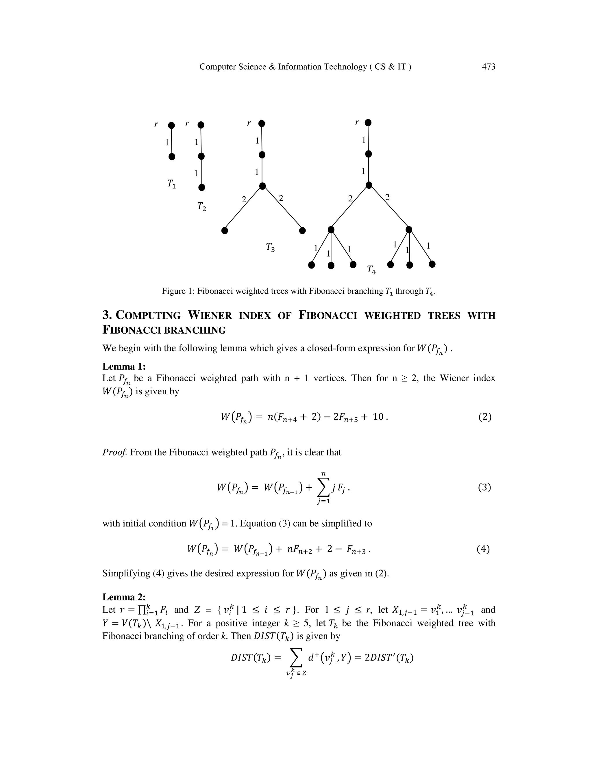
Figure 1 shows the Fibonacci weighted trees with Fibonacci branching ܶଵ through ܶସ.](https://image.slidesharecdn.com/csit2346-180203050212/75/COMPUTING-WIENER-INDEX-OF-FIBONACCI-WEIGHTED-TREES-2-2048.jpg)
![478 Computer Science & Information Technology ( CS & IT )
REFERENCES
[1] F. Buckley and F. Harary, (1990) “Distance in Graphs” (Addison-Wesley, Redwood, Vol. 42.
[2] T. H. Cormen, C.E. Leiserson, R.L. Rivest, and C. Stein, (2001) Introduction to Algorithms, McGraw-
Hill, 2nd
edition.
[3] P. Dankelmann, S. Mukwembi, and H. C. Swart, (2009) “Average distance and vertex connectivity”, J.
Graph Theory, Vol. 62(2), pp 157-177.
[4] R.C. Entringer, D.E. Jackson and D. A. Snyder, (1976) “Distance in graphs”, Czech. Math. J., Vol. 26,
pp 283-296.
[5] I. Gutman, (1988) “On distances in some bipartite graphs”, Publ. Inst. Math., (Beograd), Vol. 43, pp 3-
8.
[6] F. Harary, (1959) “Status and contrastatus”, Sociometry, Vol. 22, pp 23-43.
[7] S. Klavzar, and I. Gutman, (1997) “Wiener number of vertex-weighted graphs and chemical
applications”, Discrete Appl. Math., Vol. 80, pp 73-81.
[8] J. Plesnik, (1984) “On the sum of distances in graphs or digraph”, J. Graph Theory, Vol. 8, pp 1-21.
[9] S.G. Wagner, H. Wang, and G. Yu, (2009) “Molecular Graphs and the Inverse Wiener Index Problem”,
Discrete Appl. Math., Vol. 157, pp 1544-1554.
[10] Y. N. Yeh and I. Gutman, (1994) “On the sum of all distances in composite graphs”, Discrete Math.,
Vol. 135, pp 359-365.
AUTHORS
K. R. Udaya Kumar Reddy completed his Diploma in Computer Science and Engineering from
Siddaganga Polytechnic, Tumkur, Bangalore University in 1993. In 1998 he completed his Bachelor of
Engineering in Computer Science and Engineering from Golden Valley Institute of Technology (now Dr.
TTIT), K.G.F, Bangalore University, India. In 2004 he completed his Master of Engineering in Computer
Science and Engineering from University Visvesvaraya College of Engineering, Bangalore, India. In 2012,
he completed his Ph.D in the area of Graph Algorithms in Computer Science and Engineering, National
Institute of Technology, Trichy, India (formerly Regional Engineering College). He held various positions
at B.N.M. Institute of Technology, Bangalore, India, before joining Ph.D course and is currently a
Professor at B.N.M. Institute of Technology, Bangalore, India. His fields of interests are Algorithmic graph
theory and Theory of computation.
Ranjana S. Chakrasali received her graduation in Computer Science & Engineering from Tontadarya
College of Engineering, Gadag, Visvesvaraya Technological University (VTU), Belgaum, India in 2002.
Thereafter entered into teaching profession as a Lecturer and worked for 6 years. Currently pursuing post
graduate at BNM Institute of Technology, Bangalore, India, affiliated to VTU. Her areas of interests are
Graph Theory, Computer Graphics and Computer Networks.](https://image.slidesharecdn.com/csit2346-180203050212/75/COMPUTING-WIENER-INDEX-OF-FIBONACCI-WEIGHTED-TREES-8-2048.jpg)