Computer Networks: Unit 3 Routing protocol.ppt

CS6551 Computer Networks
Unit 3 : Routing
Dr. R.Perumalraja, Professor & Head
Department of Information Technology, VCET.
CS6551 Computer Networks, Unit 3 : Routing

Topics to be covered
 Routing
 RIP, OSPF, metrics
 Switch basics
 Global Internet
 Areas, BGP, EGP, IPv6
 Multicast addresses and Multicast routing
 DVMRP, PIM
2

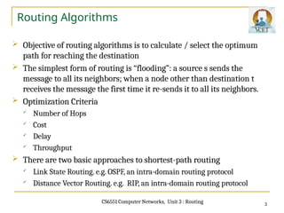
Routing Algorithms
 Objective of routing algorithms is to calculate / select the optimum
path for reaching the destination
 The simplest form of routing is “flooding”: a source s sends the
message to all its neighbors; when a node other than destination t
receives the message the first time it re-sends it to all its neighbors.
 Optimization Criteria
 Number of Hops
 Cost
 Delay
 Throughput
 There are two basic approaches to shortest-path routing
 Link State Routing. e.g. OSPF, an intra-domain routing protocol
 Distance Vector Routing. e.g. RIP, an intra-domain routing protocol
3

Routing process at a router
 Contains Routing and Forwarding Table (FT)
 Destination address based forwarding
 RT is to identify the next-hop node
 FT is to identify the Outgoing interface of next node
 Longest prefix matching
Routing Table
4
DA=my_add or
DA= IP brdcst add.
?
RT entry =
complete DA?
RT entry =
Destn. n/w id?
Default entry
exists?
No
No
No
No
Yes
Yes
Yes
Yes
Deliver datagram to
protocol module
(TCP/UDP) specified
in IP hdr.
Send pkt. to next-hop
router or to directly
connected interface.
Send pkt. to next-hop
router or to directly
connected interface.
Send pkt. to
next-hop router.
Datagram undeliverable. (Use ICMP to inform source.)
Receive incoming pkt.
DA Next hop
router
Network
Interface
Host entry 198.168.7.3 X 2
Host entry 198.168.7.4 X 3
Host entry 198.168.7.1 198.168.7.5 1
Host entry 198.168.7.2 198.168.7.5 1
N/w entry 198.100.x.x 198.100.9.1 4
N/w entry 128.72.x.x 128.72.55.4 5
Default x.x.x.x 128.84.73.1 6

Routing process example at a router
5
 How do routers build their routing tables?
 By exchanging information with each other using routing protocols
DA = 198 100 9 75
Packet generated
198.168.7.4
198.168.7.3
198.168.7.1
198.168.7.2
198.168.7.5
198.168.7.6
198.100.x.x
198.100.9.1
128.72.x.x
128.72.55.4
128.84.x.x
128.84.73.1
2
3
4
5
6
1
198.100.9.75
DA Next hop
router
N/w
Int.
Host entry 198.168.7.3 X 2
Host entry 198.168.7.4 X 3
Host entry 198.168.7.1 198.168.7.5 1
Host entry 198.168.7.2 198.168.7.5 1
N/w entry 198.100.x.x 198.100.9.1 4
N/w entry 128.72.x.x 128.72.55.4 5
Default x.x.x.x 128.84.73.1 6
Routing table (RT) at 198 168 7 6
Longest prefix match in
RT gives next hop router
as 198 100 9 1 and
outgoing interface as 4

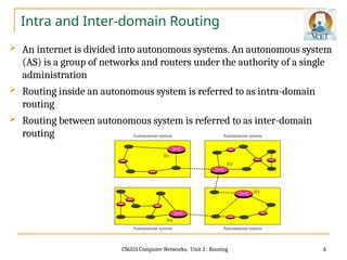
Intra and Inter-domain Routing
 An internet is divided into autonomous systems. An autonomous system
(AS) is a group of networks and routers under the authority of a single
administration
 Routing inside an autonomous system is referred to as intra-domain
routing
 Routing between autonomous system is referred to as inter-domain
routing
6

Distance Vector Routing
 a.k.a. bellman-ford algorithm
 In distance vector routing, each node maintains a table for the least cost
route between any two nodes with minimum distance
 Initially, each node knows the distance (cost) to each of its directly
connected neighbors.
 Nodes construct a vector (Destination, Cost, NextHop) and distributes
it to neighbors.
 Nodes update/compute routing table to every other node via NextHop
using the information obtained from its neighbors.
 Each node shares its routing table with its immediate neighbors
periodically and when there is a change.
 Distance vector routing is distributed, i.e., algorithm is run
7

Initialization
 At the beginning, each node can know only the distance between itself
and its immediate neighbors, those directly connected to it
8

Routing Update
Routing Update takes place in 3 steps:
The receiving node needs to add the cost between itself and the sending
node to each value in the second column of RT
Add the name of the sending node in the 3rd
column, if the receiving node
uses the information because sending node is the next node in the route
Receiving node compare and update each row of its old table with the
corresponding row of the received table.
 If the next-node entry is different, the receiving node chooses the row with
the smaller cost. If there is a tie, Kept the old one
 If the route distance is infinity, the receiving node chooses the new row. For
example, if node C has previously advertised a route to node X with distance
3. Suppose if there is no path between C and X, node C now advertises this
route with a distance of infinity. Node A must not ignore this value even
though its old entry is smaller.
9

Routing Update
10

Routing for a Small Autonomous System
11
Routing Table at Initial
Stage
Routing Table at Final
Stage

Count-to-infinity or loop instability problem
 Suppose link from node A to E goes down. 2
 Node A advertises a distance of ∞ to E to its neighbors.
 Node B receives periodic update from C before A’s update reaches B,
 Node B updated by C, concludes that E can be reached in 3 hops via C.
 Node B advertises to A as 3 hops to reach E
 Node A in turn updates C with a distance of 4 hops to E and so on.
 Thus nodes update each other until cost to E reaches infinity, i.e., no
convergence.
 Routing table does not stabilize. This problem is called loop instability
or count to infinity
12

Count-to-infinity (contd.)
13

Solutions to two-node instability
14
 Defining Infinity. In DV protocol, define the distance between each
node to be 1 and define 16 as infinity. Therefore, the distance vector
cannot be used in large systems
 Split Horizon. When a node updates its neighbors, it does not send
those routes it learned from each neighbor back to that neighbor. This
is known as split horizon.
 Split Horizon and Poison Reverse. It allows nodes to advertise
routes it learnt from a node back to that node, but with a warning
message
 Now the node B can still advertise the value of X, but if the source of
information is A, it can replace the distance with infinity as a warning:

Solutions to two node instability - Defining
Infinity
15
Defining
Infinity –
path max.
cost is 16

Routing Information Protocol (RIP)
16
 RIP is an intra-domain routing protocol based on
distance-vector algorithm
 Routers advertise the cost of reaching networks.
Cost of reaching each link is 1 hop.
 Each router updates cost and next hop for each
network number.
 Infinity is defined as 16, i.e., any route cannot
have more than 15 hops. Therefore RIP can be
implemented on small-sized networks only.
 Advertisements are sent every 30 seconds or in
case of triggered update.
 RIP packet format (version 2) contains (network
address, distance) pairs.

Routing Update example
 Update message sent from router R1 to router R2 through 130.10.0.2
17
The message is prepared with the
combination of split horizon and
poison reverse strategy in mind.

Timer in RIP
18
 RIP uses 3 timers. The periodic timer controls the sending of messages,
the expiration timer governs the validity of a route, and the garbage
collection timer advertises the failure of a route
 Every time a new update for the route is received, Expiration timer is
reset to 180. If the timer is expired, the hop count of the route is set to
16, which means the destination is unreachable
 When the information about a route becomes invalid, the router does
not immediately purge that route from its table Instead, it continues to
advertise the route with a metric value of 16 until the Garbage timer
reaches to 0

RIP: link failure, recovery
 If no advertisement heard after 180 sec  neighbor/link declared as
dead
 routes via neighbor invalidated
 new advertisements sent to neighbors
 neighbors in turn send out new advertisements (if tables changed)
 link failure info quickly (?) propagates to entire net
 Poison reverse is used to prevent ping-pong loops (infinite distance =
16 hops)
19

RIP Timer - Example
 A routing table has 20 entries. It does not receive information about
five routes for 200 s. How many timers are running at this time?
 Solution: The 21 timers are listed below
 Periodic timer: 1
 Expiration timer: 20−5= 15
 Garbage collection timer: 5
20

Link State Routing
 Open Shortest Path First (OSPF) algorithm uses the Link State Protocol,
developed by IETF IGP working group, RFC2328
 In LSR, each node knows state of link to its neighbors and cost. Hence,
each router floods link-state information through its neighbors to other
routers
 Based on the flooded link-state information, each router maintains a
complete link-state database
 Based on the link-state database, a routing table is constructed using
SPF (e.g., Dijkstra’s) algorithm
 Link-state routing relies on two mechanisms
 Reliable flooding−distribution of Link State Path (LSP) to all other nodes
 Forward Search algorithm−Route calculation from accumulated LSPs.
21

Reliable Flooding
 Nodes create an update packet called link-state packet (LSP) and sends
out on each of its links, that contains :
 ID of the node
 List of neighbors for that node and associated cost
 64-bit Sequence number
 Time to live
 When a node receives a LSP, checks if it has an LSP already for that node
 If not, it stores that LSP, else it keeps the LSP with larger sequence number.
 Forwards the LSP on all other links except the incoming one.
 Thus recent LSP of a node reaches all nodes, i.e., reliable flooding
 LSP is generated either periodically or when there is a change in the n/w
topology
22

Reliable Flooding & Forward Search
Forward Search
Each node computes the route after it has received LSPs of other nodes, using
a variation of Dijkstra’s algorithm, known as forward search algorithm.
Nodes maintain two lists, namely Tentative and Confirmed with entries of
the form (Destination, Cost, NextHop).
23
Reliable Flooding

Forward Search Algorithm
Algorithm
•Initialize the Confirmed list with an entry for
the Node (Cost = 0).
•Node just added to Confirmed list is called
Next. Its LSP is examined.
•For each neighbor of Next, calculate cost to
reach each neighbor: Cost (Node to Next) +
Cost (Next to Neighbor).
•If Neighbor is not in any list, then add
(Neighbor, Cost, NextHop) to Tentative list.
•If Neighbor is in Tentative list, then retain
entry with the least cost.
•If Tentative list is empty then Stop,
•Move least cost entry from Tentative list to
Confirmed list. Go to Step 2.
24
Step Confirmed Tentative Comment (routing table for node D)
1 (D, 0, –) D is moved to Confirmed list initially
2 (D, 0, –)
(B, 11, B)
(C, 2, C)
Based on D's LSP, its immediate
neighbors B and C are
added to Tentative list
3
(D, 0, –)
(C, 2, C)
(B, 11, B)
Lowest cost entry C in Tentative list is
moved to Confirmed
list. C's LSP is to be examined next
4
(D, 0, –)
(C, 2, C)
(B, 5, C)
(A, 12, C)
Cost to reach B through C is 5, so the
entry (B, 11, B) is
replaced. C's neighbor A is also added
to Tentative list
5
(D, 0, –)
(C, 2, C)
(B, 5, C)
(A, 12, C)
Lowest cost entry B is moved to
Confirmed list. B's LSP is
examined next.
6
(D, 0, –)
(C, 2, C)
(B, 5, C)
(A, 10, C)
Since A could be reached through B at
a lower cost than the
existing one, the Tentative list entry
(A, 12, C) is replaced to
(A, 10, C)
7
(D, 0, –)
(C, 2, C)
(B, 5, C)
(A, 10, C)
Node A is moved to Confirmed list.
Process completed, since
tentative list has no entries

Features of OSPF
 Use flexible metrics instead of only hop count
 Supports variable-length subnetting
 Supports multiple routes; one for each IP type of service (ToS)
 Quick convergence
 Uses multicast rather than broadcast of its messages to reduce network
load
 Authentication―Routing updates are authenticated to prevent
malicious nodes from providing false costs.
 Scalable: OSPF is more scalable using network hierarchy w.r.t areas
 Load balancing―Traffic is evenly distributed by assigning uniform cost
to various routes to a destination.
25

Hierarchical OSPF
 AS is organized as two-level
hierarchy
 AS is partitioned into self-contained
areas
 Areas are interconnected by a
backbone area
 Areas are identified by a 32-bit area
ID
 0.0.0.0 is reserved for the backbone
area
 Four types of routers
 Internal router, area border router,
backbone router, autonomous
system boundary router (ASBR)
26

OSPF Operations
 Hello protocol
 Hello packets are transmitted to all interfaces periodically
 Discover neighbors, establish and maintain neighbor adjacency relationships
 Elect Designated Router (DR) if multiple routers are in a broadcast network
 Database synchronization
 Two neighboring routers exchange database description packets to
synchronize their link-state databases.
 Database description includes only a list of LSA headers. New or more up-to-
date LSAs will be requested later
 Propagation of link-state information: Reliable Flooding
 Building of routing table: Routing algorithm may use Forward Search
27

Routing metrics
 Hop (Uniform cost to all links)
 Easy to calculate least-cost route.
 Latency, Bandwidth, etc., are not considered. For eg. links with latency 250 ms and
1 ms ; links with BW 1 Mbps and 100 Mbps are treated similarly
 Original ARPANET (queue length as its routing metric)
 Higher cost was assigned for links with long queue than shorter ones.
 Packets moved towards short queues, but not towards destination.
 Bandwidth and latency were not considered.
 ARPANETs new routing mechanism was as follows
 Bandwidth, latency and delay was used to estimate load, rather than queue
length.
 ArrivalTime and DepartTime of a packet at a router was recorded.
 Weights were assigned to links based on avg. delay for packets over that link.
28

Limitations of IPV4 & Advantages of IPV6
 Limitations of IPV4
 Despite subnetting and CIDR, address depletion is still a long-term problem.
 Internet must accommodate real-time audio and video transmission that
requires minimum delay strategies and reservation of resources.
 Internet must provide encryption and authentication of data for some
applications.
 Advantages of IPv6 over IPv4
 Address space―IPv6 uses 128-bit address whereas IPv4 uses 32-bit address.
Hence IPv6 has huge address space than IPv4
 Header format―Unlike IPv4, optional headers are separated from base
header in IPv6. Each router thus need not process unwanted information
 Extensible―Unassigned IPv6 addresses can accommodate needs of future
technologies.
29

Features of IPV6
 IPv6 solved address space exhaustion in IPv4 and offers rich set of
services
 128-bit addresses to handle up to 3.4 ×1038 nodes
 IPv6 uses classless addressing, but classification is based on MSBs
 IPv6 unicast addresses start with 001 prefix
 Multicast start with a byte of 1s
 Reserved addresses start with a byte of 0s
 Support real-time services
 Enhanced Authentication and security
 End-to-end fragmentation
 Enhanced routing functionality, including support for mobile hosts
30

IPV6 Addressing
 Classless addressing/routing (similar to CIDR)
 Notation: x:x:x:x:x:x:x:x(x= 16-bit hex number)
 Contiguous 0s are compressed: 47CD::A456:0124
 IPv6 compatible IPv4 address: ::128.42.1.87
 Address assignment
 Provider based and geographic based.
 Address Aggregation
 IPv6 provides aggregation by assigning prefixes at continental level to reduce
routing table entries. For example, addresses in Europe to have a common
prefix, then routers in other continents would need one routing table entry
for all networks in Europe..
31

IPV6 Header
 Base header is 40 bytes long
 Version – specifies the IP version, i.e., 6.
 TrafficClass – defines priority of the packet with
respect to traffic congestion.
 FlowLabel – provides special handling for a
particular flow of data.
 PayloadLen – gives length of the packet,
excluding header.
 NextHeader – contains a pointer to optional
headers following IP header.
 HopLimit – specifies lifetime of the packet.
 SourceAddress / DestinationAddress – 16-byte
addresses of source and destination host
32

Extension Headers of IPV6
 Base header may be followed by six extension headers in specific order.
 Each extension header contains a NextHeader field to identify the header
following it.
 Hop-by-Hop – source host passes information to all routers
 Source Routing -routing information (strict/loose) provided by the source
 Fragmentation
 Authentication – used to validate the sender and ensures data integrity
 Security for Payload - provides confidentiality against eavesdropping
 Destination - source host information is passed to the destination only
33

Thank you
34

Computer Networks: Unit 3 Routing protocol.ppt

More Related Content

Similar to Computer Networks: Unit 3 Routing protocol.ppt

More from hodai16

Recently uploaded

Computer Networks: Unit 3 Routing protocol.ppt