This document summarizes and compares different methods for aiding decision makers in selecting preferred solutions from large sets of Pareto optimal solutions in multi-objective optimization problems. It focuses on two main methods: 1) an a priori method called Guided Multi-Objective Genetic Algorithm (G-MOGA) and 2) an a posteriori method using subtractive clustering and fuzzy preference assignment. These methods are compared using a case study involving optimization of test intervals for components in a nuclear power plant safety system with objectives of availability, cost, and worker exposure. The document provides background on the case study problem and objectives before analyzing and comparing the different decision support methods.

1. Chapter 2
A Comparison of Methods For Selecting
Preferred Solutions in Multiobjective Decision
Making
Enrico Zio1,2 and Roberta Bazzo2
1 Chair “Systems Science and Energetic Challenge” European Foundation for New
Energy – EDF, École Centrale Paris – Supelec, Paris, France
2 Dipartimento di Energia, Politecnico di Milano, Milano, Italy
E-mail: enrico.zio@ecp.fr, enrico.zio@supelec.fr, enrico.zio@polimi.it
In multiobjective optimization problems, the identified Pareto Frontiers and Sets often con-
tain too many solutions, which make it difficult for the decision maker to select a preferred
alternative. To facilitate the selection task, decision making support tools can be used in
different instances of the multiobjective optimization search to introduce preferences on
the objectives or to give a condensed representation of the solutions on the Pareto Frontier,
so as to offer to the decision maker a manageable picture of the solution alternatives.
This paper presents a comparison of some a priori and a posteriori decision making support
methods, aimed at aiding the decision maker in the selection of the preferred solutions.
The considered methods are compared with respect to their application to a case study
concerning the optimization of the test intervals of the components of a safety system of
a nuclear power plant. The engine for the multiobjective optimization search is based on
genetic algorithms.
2.1 Introduction
Multiobjective optimization is central for many reliability and risk analyses in support
to the design, operation, maintenance and regulation of complex systems like nuclear power
plants. The solutions sought must be optimal with respect to several objectives, generally
conflicting: then, one cannot identify a unique, optimal solution satisfying all objectives,
but rather a set of possible solutions can be identified where none is best for all objectives.
This set of solutions in the space of the decision variables is called the Pareto Set; the
corresponding values of the objectives form the Pareto Frontier.
C. Kahraman (ed.), Computational Intelligence Systems in Industrial Engineering, 23
Atlantis Computational Intelligence Systems 6, DOI: 10.2991/978-94-91216-77-0_2,
Ó Atlantis Press 2012

2. 24 Computational Intelligence Systems in Industrial Engineering
At the end of a multiobjective optimization, the decision maker (DM) has to select the
preferred solutions from the Pareto Frontier and Set; this can be a difficult task for large
Pareto Frontiers and Sets. For this reason, decision making support tools are developed to
aid the DM in selecting the preferred solutions.
There are different approaches for introducing DM preferences in the optimization pro-
cess, like the ones presented by ATKOSoft [1], Rachmawati and Srinivasan [14], and Coello
Coello [6]; a common classification is based on when the DM is consulted: a priori, a pos-
teriori, or interactively during the search.
In this work, a comparison of some a prioripriori methods and a posteriori methodspos-
teriori methods is performed, aimed at characterizing the different approaches in terms of
their advantages and limitations with respect to the support they provide to the DM in the
preferential solution selection process; to this purpose, not just the quality of the results, but
also the possible difficulties of the DM in applying the procedures are considered. In or-
der to base the comparison on solid experience, the methods considered have been chosen
among some of those most extensively researched by the authors.
The a priori method considered is the Guided Multi-Objective Genetic Algorithm (G-
MOGA) by Zio, Baraldi and Pedroni [18], in which the DM preferences are implemented
in a genetic algorithm to bias the search of the Pareto optimal solutions.
The first a posteriori method considered has been introduced by the authors [20] and
uses subtractive clustering [5] to group the Pareto solutions in homogeneous families; the
selection of the most representative solution within each cluster is performed by the analy-
sis of Level Diagrams [2] or by fuzzy preference assignment [19], depending on the decision
situation, i.e., depending on the presence or not of defined DM preferences on the objec-
tives. The second procedure, is taken from literature [11] and is a two-step procedure which
exploits a Self Organizing Map (SOM) [8] and Data Envelopment Analysis (DEA) [7] to
first cluster the Pareto Frontier solutions and then remove the least efficient ones. This
procedure is here only synthetically described and critically considered with respect to the
feasibility of its application in practice.
Instead, the a priori G-MOGA algorithm and the first a posteriori procedure introduced
by the authors in [20], are compared with respect to a case study of literature regarding
the optimization of the test intervals of the components of a nuclear power plant safety
system; the optimization considers three objectives: system availability to be maximized,
cost (from operation & maintenance and safety issues) and workers exposure time to be

3. A Comparison of Methods For Selecting Preferred Solutions in Multiobjective Decision Making 25
minimized [9]. The a posteriori procedure of analysis is applied to the Pareto Frontier and
Set obtained by a standard Multiobjective Genetic Algorithm [9].
The remainder of the paper is organized as follows: Section 2.2 presents the case study
to describe upfront the setting of the typical multiobjective optimization problem of in-
terest; Section 2.3 contains the analysis of the different decision making support methods
considered; finally some conclusions are drawn in Section 2.4.
2.2 Optimization of the test intervals of the components of a nuclear power
plant safety system
The case study here considered is taken from Giuggioli Busacca, Marseguerra and
Zio [9] and regards the optimization of the test intervals (TIs) of the high pressure injection
system (HPIS) of a pressurized water reactor (PWR), with respect to three objectives: mean
system availability to be maximized, cost and workers time of exposure to radiation to be
minimized. For reader’s convenience, the description of the system and of the optimiza-
tion problem is here reported, as taken from the original literature source with only minor
modifications.
Fig. 2.1 The simplified HPIS system (RWST = radioactive waste storage tank) [9]
Figure 2.1 shows a simplified schematics of a specific HPIS design. The system con-
sists of three pumps and seven valves, for a total of Nc = 10 components. During normal
reactor operation, one of the three charging pumps draws water from the volume control
tank (VCT) in order to maintain the normal level of water in the primary reactor cooling
system (RCS) and to provide a small high-pressure flow to the seals of the RCS pumps.
Following a small loss of coolant accident (LOCA), the HPIS is required to supply a high

4. 26 Computational Intelligence Systems in Industrial Engineering
pressure flow to the RCS. Moreover, the HPIS can be used to remove heat from the reactor
core if the steam generators were completely unavailable. Under normal conditions, the
HPIS function is performed by injection through the valves V3 and V5 but, for redundancy,
crossover valves V4 , V5 and V7 provide alternative flow paths if some failure were to occur
in one of the nominal paths. This stand-by safety system has to be inspected periodically
to test its availability. A TI of 2190 h is specified by the technical specifications (TSs) for
both the pumps and the valves. However, there are several restrictions on the maintenance
procedures described in the TS, depending on reactor operations.
For this study, the following assumptions are made:
(1) At least one of the flow paths must be open at all times.
(2) If the component is found failed during surveillance and testing, it is returned to an
as-good-as-new condition through corrective maintenance or replacement.
(3) If the component is found to be operable during surveillance and testing, it is returned
to an as-good-as-new condition through restorative maintenance.
(4) The process of test and testing requires a finite time; while the corrective maintenance
(or replacement) requires an additional finite time, the restorative maintenance is sup-
posed to be instantaneous.
The Nc system components are characterized by their failure rate λh , h = 1, . . . , Nc , the
cost of the yearly test Cht,h and corrective maintenance Chc,h , the mean downtime due to
corrective maintenance dh , the mean downtime due to testing th and their failure on demand
probability ρh (Table 2.1). They are also divided in three groups characterized by different
test strategies with respect to the TI τh between two successive tests, h = 1, . . . , Nc , Nc = 10;
all the components belonging to a same group undergo testing with the same periodicity
T g , with g = 1, 2, 3, i.e., they all have the same test interval (τh = T g , ∀ component h in
test group g).
Any solution to the optimization problem can be encoded using the following array θ
of decision variables:
θ = T1 T2 T3 (2.1)
Assuming a mission time (TM) of one year (8760 h), the range of variability of the
three TIs is [1, 8760] h.
The search for the optimal test intervals is driven by the following three objective func-
tions Ji (θ ), i = 1, 2, 3:

5. A Comparison of Methods For Selecting Preferred Solutions in Multiobjective Decision Making 27
Table 2.1 Characteristics of the system components
Component
Component λh Cht,h Chc,h
symbol dh (h) th (h) ρh g
( j) (h−1 ) ($/h) ($/h)
(Figure 2.1)
1 V1 5.83 · 10−6 20 15 2.6 0.75 1.82 · 10−4 1
2 V2 5.83 · 10−6 20 15 2.6 0.75 1.82 · 10−4 1
3 V3 5.83 · 10−6 20 15 2.6 0.75 1.82 · 10−4 2
4 V4 5.83 · 10−6 20 15 2.6 0.75 1.82 · 10−4 3
5 V5 5.83 · 10−6 20 15 2.6 0.75 1.82 · 10−4 2
6 V6 5.83 · 10−6 20 15 2.6 0.75 1.82 · 10−4 3
7 V7 5.83 · 10−6 20 15 2.6 0.75 1.82 · 10−4 3
8 PA 3.89 · 10−6 20 15 24 4 5.3 · 10−4 2
9 PB 3.89 · 10−6 20 15 24 4 5.3 · 10−4 2
10 Pc 3.89 · 10−6 20 15 24 4 5.3 · 10−4 2
Mean Availability, 1 − U HPIS :
NMCS nv
max J1 (θ ) = max
θ θ
1− ∑ ∏ uv (θ )
h (2.2)
v=1 h=1
Nc
Cost, C: min J2 (θ ) = min Caccident (θ ) + ∑ CS&M,h (θ ) (2.3)
θ θ h=1
Nc
Exposure Time, ET : min J3 (θ ) = min
θ θ
∑ ETh (θ ) (2.4)
h=1
For every solution alternative θ :
the HPIS mean unavailability U HPIS (θ ) is computed from the fault tree for the top
event “no flow out of both injection paths A and B” [9]; the boolean reduction of the corre-
sponding structure function allows determining the NMCS system minimal cut sets (MCS);
then, the system mean unavailability is expressed as in the argument of the maximization
(2.2), where nv is the number of basic events in the v-th minimal cut set and uv is the mean
h
unavailability of the h-th component contained in the v-th MCS, h = 1, . . . , nv [12]:
1 dh th
uv = ρh + λh τh + (ρh + λhτh ) + + γ0 (2.5)
h
2 τh τh
where γ0 is the probability of human error. The simple expression in (2.5) is valid for ρh <
0.1 and λh τh < 0.1, which are reasonable assumptions when considering safety systems.
the cost objective C(θ ) is made up of two major contributions: CS&M (θ ), the cost
associated with the operation of surveillance and maintenance (S&M) and Caccident (θ ), the
cost associated with consequences of accidents possibly occurring at the plant.

6. 28 Computational Intelligence Systems in Industrial Engineering
For a given component h, the S&M cost is computed on the basis of the yearly test and
corrective maintenance costs. For a given mission time, TM, the number of tests performed
on component h are TM
τh ; of these, on average, a fraction equal to (ρh + λhτh ) demands also
a corrective maintenance action of duration dh ; thus, the S&M costs amount to:
TM TM
CS&M,h (θ ) = Cht,h th + Chc,h (ρh + λh τh ) dh , h = 1, . . . , Nc (2.6)
τh τh
Concerning the accident cost contribution, it is intended to measure the costs associated
to damages of accidents which are not mitigated due to the HPIS failing to intervene. A
proper analysis of such costs implies accounting for the probability of the corresponding
accident sequences; for simplicity, but with no loss of generality, consideration is here
limited only to the accident sequences relative to a small LOCA event tree [17] (Figure 2.2).
Fig. 2.2 Small LOCA event tree [17]
The accident sequences considered for the quantification of the accident costs are those
which involve the failure of the HPIS (thick lines in Figure 2.2), so that the possible Plant
Damage States (PDS) are PDS1 and PDS3. Thus:
⎧
⎪ Caccident = C1 + C3
⎪
⎨
C = P(EI) · (1 − URT ) ·U HPIS · {ULPIS + (1 − ULPIS ) ·USDC ·UMSHR } ·CPDS1
⎪ 1
⎪
⎩ C = P (EI) · (1 − U ) ·U
3 RT HPIS · (1 − ULPIS ) · {(1 − UMSHR ) ·USDC + (1 − USDC )} ·CPDS3
(2.7)
where C1 and C3 are the total costs associated with accident sequences leading to damag-
ing states 1 and 3, respectively. These costs depend on the initiating event frequency P(EI)

7. A Comparison of Methods For Selecting Preferred Solutions in Multiobjective Decision Making 29
Table 2.2 Accident cost input data [9]
P(EI) URT ULPIS USDC UMSHR CPDS1 CPDS2
(y−1 ) (y−1 ) (y−1 ) (y−1 ) (y−1 ) ($×event) ($×event)
2.43 · 10−5 3.6 · 10−5 9 · 10−3 5 · 10−3 5 · 10−3 2.1765 · 109 1.375 · 108
Table 2.3 MOGA input parameters and rules [9]
Number of chromosomes (Np ) 100
Number of generations (termination criterion) 500
Selection Standard Roulette
Replacement Random
Mutation probability 5 · 10−3
Crossover probability 1
Number of non-dominated solutions in the archive 100
and on the unavailability values Ui of the safety systems which ought to intervene along
the various sequences: these values are taken from the literature [13, 17]. Rates of Initiat-
ing Events at United States Nuclear Power Plants: 1987-1995) for all systems except for
the SDC and MSHR, which were not available and were arbitrarily assumed of the same
order of magnitude of the other safety systems, and for the HPIS for which the unavailabil-
ity U HPIS is calculated from (2.2) and (2.5) and it depends on the TIs of the components.
Finally, for the values of CPDS1 and CPDS3 , the accident costs for PDS1 and PDS3, respec-
tively, are taken as the mean values of the uniform distributions given in Yang, Hwang,
Sung and Jin [17]. Table 2.2 summarizes the input data.
the exposure time ET due to the tests and possible maintenance activities on a single com-
ponent h can be computed as:
TM TM
ETh (θ ) = th + (ρh + λhτh ) dh , h = 1, . . . , Nc (2.8)
τh τh
Then,
Nc
ET (θ ) = ∑ ETh(θ ) (2.9)
h=1
The multiobjective optimization problem (2.2)–(2.4) has been solved using the MOGA
code developed at the Laboratorio di Analisi di Segnale e Analisi di Rischio (LASAR,
Laboratory of Signal Analysis and Risk Analysis, http://lasar.cesnef.polimi.it/);
the input parameters and settings are reported in Table 2.3 [9].
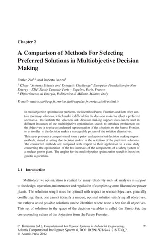
The resulting Pareto Set (Θ) is made of 100 points, and the corresponding Pareto Fron-
tier is showed in Figure 2.3 in the objective functions space.

8. 30 Computational Intelligence Systems in Industrial Engineering
Fig. 2.3 Pareto Frontier, in the objective functions space, obtained by the MOGA code
2.3 Decision support methods
2.3.1 A posteriori approaches
When analyzing the Pareto Frontier, the DM either:
• looks for the solution closest to the ideal one, i.e., that which optimizes all the objec-
tives simultaneously;
• applies his or her preferences on the objective functions values to identify the best
solution according to these preferences.
The two decision situations, i.e., in presence or not of preferences on the objectives
values, may lead to the selection of different solutions and require different procedures of
reduction of the solutions in the Pareto Frontier. To this purpose, different a posteriori
procedures can be developed to aid the DM in selecting the preferred solution; two of these
are synthetically illustrated in the following.
The first a posteriori method presented below, is based on a two-step procedure devel-
oped by the authors, for which the availability of the software has rendered possible the
comparison on a literature case study.
The second method based on the Self Organizing Maps and Data Envelopment Analysis
has been proposed elsewhere in the literature and its application is here critically evaluated.

9. A Comparison of Methods For Selecting Preferred Solutions in Multiobjective Decision Making 31
2.3.1.1 Subtractive clustering, fuzzy scoring and Level Diagrams for decision
making support [20]
A two-step procedure has been introduced by the authors in Zio and Bazzo [20]. This
procedure consists in grouping in “families” by subtractive clustering the non-dominated
solutions of the Pareto Set, according to their geometric relative distance in the objective
functions space (Pareto Frontier), and then selecting an “head of the family” representa-
tive solution within each cluster. Level Diagrams [2] are used to effectively represent and
analyze the reduced Pareto Frontiers; they account for the distance of the Pareto Frontier
and Set solutions from the ideal (but not feasible) solution, optimal with respect to all the
objectives simultaneously.
Considering a multiobjective problem with l objectives to be minimized, m to be max-
imized (such that Nobj = l + m), n solutions in the Pareto Set, and indicating by J θ i =
J1 θ i . . . Js θ i . . . JNobj θ i the objective functions values vector corresponding to
the solution θi in the Pareto Set Θ, i = 1, . . . , n, the distance of each Pareto solution from
the optimal solution can be measured in terms of the following 1-norm:
Nobj
1-norm: J θi 1
= ∑ Js,norm θ i , with 0 J θi 1
s, s = 1, . . . , Nobj (2.10)
s=1
where each objective value Js θ i , is normalized with respect to its minimum and maxi-
mum values (Js and Js ) on the Pareto Frontier [2] as follows:
min max
Js θ i − Jsmin
Js,norm θ i = max − J min
, s = 1, . . . , l (2.11)
Js s
and
Js − Js θ i
max
Js,norm θ i = , s = 1, . . . , m (2.12)
Js − Js
max min
Subtractive clustering operates on the normalized objective values J norm θ i , i =
1, . . . , n and groups the non-dominated solutions in “families” according to their geometri-
cal distance; it starts by calculating the following potential P J norm θ i [5]:
n
4
P J norm θ i = ∑ e− α J norm (θ i )−J norm (θ l ) 2
, α= 2
(2.13)
l=1 ra
where ra , the cluster radius, is a parameter which determines the number of clusters that
will be identified. The first cluster center J 1
norm is selected as the solution with the highest
norm . All the other n−1 solutions potentials P J norm θ
potential value P J 1 i are corrected

10. 32 Computational Intelligence Systems in Industrial Engineering
subtracting the potential P J 1
norm multiplied by a factor which considers the distance be-
tween the i-th solution and the first cluster center:
−β Jnorm (θ i )−J1 2
P J norm θ i = P J norm θ i − P J1
norm e
norm ,
4
β = 2 and rb = qra (2.14)
rb
where q is an input parameter called squash factor, which indicates the neighborhood with
a measurable reduction of potential expressed as a fraction of the cluster radius and is here
set equal to 1.25.
j
Generally, for the the j-th cluster center found J norm , j = 1, . . . , K, the potentials are reduced
as follows:
j
P J norm θ i = P J norm θ i − P J norm e−β
j Jnorm (θ i )−Jnorm 2
(2.15)
The process of finding new cluster centers and reducing the potential is repeated until a
stopping criterion is reached [5].
The cluster radius ra is chosen to maximize the quality of the resulting Pareto Frontier
partition measured in terms of the silhouette value [15, 16]; for any cluster partition of the
Pareto Frontier, a global silhouette index, GS, is computed as follows:
K
1
GS =
K ∑ Sj (2.16)
j=1
where S j is the cluster silhouette of the j-th cluster F j , a parameter measuring the hetero-
geneity and isolation properties of the cluster [15, 16], computed as the average value of
the silhouette widths s(i) of its solutions, defined as:
b(i) − a(i)
s(i) = , i = 1, . . . , n (2.17)
max{a(i), b(i)}
where n is the number of solutions in the Pareto Set, a(i) is the average distance from the
i-th solution of all the other solutions in the cluster, and b(i) is the average distance from
the i-th solution of all the solutions in the nearest neighbor cluster, containing the solutions
of minimum average from the i-th solution, on average.
A head of the family must then be chosen as the best representative solution of each
cluster. If no DM preferences are given, the solution with the lowest 1-norm value in
each cluster is chosen as the best representative solution; according to the Level Diagrams
definition, this means that the selected solution is the closest to the ideal solution, optimal
with respect to all objectives. If, on the other hand, the DM preferences on the objective
values are available, the best solutions for the DM can be assigned classes of merit with

11. A Comparison of Methods For Selecting Preferred Solutions in Multiobjective Decision Making 33
respect to the DM preferences, by setting objective values thresholds. Let us consider the
Pareto Set Θ made of n solutions; to the i-th solution θ i (i = 1, . . . , n) corresponds a vector
of objective values
J θ i = J1 θ i J2 θ i . . . JNobj θ i (2.18)
where Nobj is the number of objective functions of the optimization problem. The objective
values thresholds are given in a preference matrix P (Nobj × C), where C is the number of
objective functions thresholds used for the classification, defining C + 1 preference classes
as in Figure 2.4 [2].
Fig. 2.4 Class Thresholds assignment
where Js , Z = 1, . . . , 5, are the thresholds values of the s-th objective, l and m are the
Z
number of objectives to be minimized and maximized, respectively.
The fuzzy scoring procedure introduced by the authors in Zio and Bazzo [19] is then
applied: each preference class is assigned a score sv(r) [2], r = 1, . . . ,C + 1, such that:
sv(C + 1) = 0; sv(r) = Nobj · sv(r + 1) + 1, for r = C, . . . , 1 (2.19)
and each objective value Js θ i , i = 1, . . . , n and s = 1, . . . , Nobj , is assigned a membership
function μAr Js θ i
s
which represents the degree with which Js θ i is compatible with the
fact of belonging to the r-th preference class, r = 1, . . . ,C + 1.

12. 34 Computational Intelligence Systems in Industrial Engineering
A vector of C + 1 = 6 membership functions is then defined for each objective Js :
μ Js θ i = μA1 Js θ i μA2 Js θ i μA3 Js θ i μA4 Js θ i μA5 Js θ i μA6 Js θ i
s s s s s s
i = 1, . . . , n, s = 1, . . . , Nobj . (2.20)
The membership-weighted score of each individual objective is then computed; given
the scoring vector sv = sv(1) sv(2) . . . sv(C + 1) , whose components are defined in
(2.19), and the membership functions vector μ Js θ i in (2.20) for the i-th solution and
s-th objective function, the score svi of the individual objective Js is obtained by weighting
s
the score sv(rs ) of each class rs the objective belongs to, by the respective membership
function value μArs Js θ i , rs = 1, . . . , 6, and then summing the 6 resulting terms. This
s
can be formulated in terms of the scalar product of the vectors μ Js and sv as follows:
i
μ Js θ i , sv
svi =
s 6
, i = 1, . . . , n and s = 1, . . . , Nobj , (2.21)
∑ μ Ars
s
Js θi
rs =1
where the denominator serves as the normalization factor.
Then, the score S J θ i of the i-th solution is the sum of the scores of the individual
objectives
Nobj
S J θi = ∑ svis , i = 1, . . . , n (2.22)
s=1
and the lowest score is taken as the most preferred solution.
According to this fuzzy scoring procedure, the head H j of the generic family F j , j =
1, . . . , K, is chosen as the solution in F j with lowest scores S J θ i :
S H j = min S J θ i k
, k = 1, . . . , n j and j = 1, . . . , K (2.23)
Level Diagrams [2] are finally used to represent and analyse the reduced Pareto Frontier
thereby obtained.
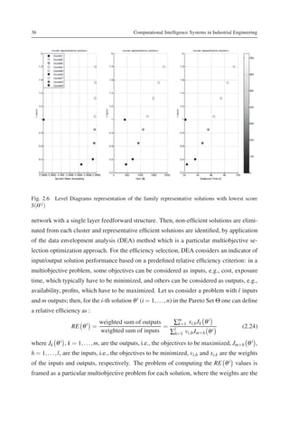
With reference to the Pareto Frontier of Figure 2.3 for the test intervals optimization
case study, the maximum value of the global silhouette (0.71) is found in correspondence
of a cluster radius equal to 0.18 , as showed in Figure 2.5, which results in K = 9 clusters.
For illustration purposes, let us introduce an arbitrary preference matrix P for the test inter-
vals optimization (Table 2.4).
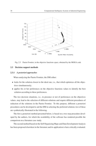
The reduced Pareto Frontier is showed in Figure 2.6: the best solutions (the dark circles)
can be easily identified; there are also 4 solutions (the white circles) which have high score
values, and thus are unacceptable, i.e., not interesting for the DM.

13. A Comparison of Methods For Selecting Preferred Solutions in Multiobjective Decision Making 35
Fig. 2.5 GS for different cluster radius values
Table 2.4 Preference threshold matrix P
1
Js 2
Js 3
Js 4
Js 5
Js
J1 0.9975 0.998 0.9985 0.999 0.9995
J2 900 800 700 600 500
J3 60 50 45 40 30
Note that for the application of the method, the DM only has to select the optimum
cluster radius (from Figure 2.5), define the preference matrix and use the Level Diagrams
representation to evaluate the solutions according to their distance from the ideal solution,
optimal with respect to all objectives.
2.3.1.2 Self-Organizing Maps solution clustering and Data Envelopment
Analysis solution pruning for decision making support [11]
Another approach to simplifying the decision making in multiobjective optimization
problems has been introduced in Li, Liao and Coit [11], based on Self Organizing Maps
(SOM) [8] and Data Envelopment Analysis (DEA) [7].
The Pareto optimal solutions are first classified into several clusters by applying the
SOM method, an unsupervised classification method based on a particular artificial neural

14. 36 Computational Intelligence Systems in Industrial Engineering
Fig. 2.6 Level Diagrams representation of the family representative solutions with lowest score
S(H j )
network with a single layer feedforward structure. Then, non-efficient solutions are elimi-
nated from each cluster and representative efficient solutions are identified, by application
of the data envelopment analysis (DEA) method which is a particular multiobjective se-
lection optimization approach. For the efficiency selection, DEA considers an indicator of
input/output solution performance based on a predefined relative efficiency criterion: in a
multiobjective problem, some objectives can be considered as inputs, e.g., cost, exposure
time, which typically have to be minimized, and others can be considered as outputs, e.g.,
availability, profits, which have to be maximized. Let us consider a problem with l inputs
and m outputs; then, for the i-th solution θ i (i = 1, . . . , n) in the Pareto Set Θ one can define
a relative efficiency as :
weighted sum of outputs ∑m xi,k Jk θ i
RE θ i = = l k=1 (2.24)
weighted sum of inputs ∑h=1 vi,h Jm+h θ i
where Jk θ i , k = 1, . . . , m, are the outputs, i.e., the objectives to be maximized, Jm+h θ i ,
h = 1, . . . , l, are the inputs, i.e., the objectives to be minimized, vi,h and xi,k are the weights
of the inputs and outputs, respectively. The problem of computing the RE θ i values is
framed as a particular multiobjective problem for each solution, where the weights are the

15. A Comparison of Methods For Selecting Preferred Solutions in Multiobjective Decision Making 37
decision variables and the relative efficiency is the objective function to be maximized:
∑m xi,k Jk θ i
max RE θ i = max k=1
(2.25)
h=1 vi,h Jm+h θ
ui,k ,vi,h ui,k ,vi,h ∑l i
The Pareto Frontier is then reduced to the solutions with the highest relative efficiency
values RE θ i and the DM is provided with a small number of most efficient solutions.
This method has been showed to be effective in reducing the number of possible so-
lutions to be presented to the DM in a multiobjective reliability allocation problem [11],
but not with the inclusion of the DM preferences. The solution selection is based only
on a solution performance criterion (the relative efficiency), but in presence of particular
requirements on the objective values, the solutions most preferred by the DM might not be
the most efficient ones. Also, the DEA method solves a maximization problem for each
solution and this increases the computational time, particularly for large Pareto Frontiers.
2.3.2 A priori approach
The a priori approach considered in this work is the Guided Multiobjective Genetic
Algorithm (G-MOGA) [18]. The deep knowledge of this method co-developed by one of
the authors, makes it a suitable a priori method for detailed comparison on the literature
case study.
DM preferences are taken into account by modifying the definition of dominance used
for the multiobjective optimization [3, 4]. In general, dominance is determined by pair-
wise vector comparisons of the multiobjective values corresponding to the pair of solutions
under comparison; specifically, solution θ 1 dominates solution θ 2 if
∀ i ∈ {1, . . . , s}, Ji θ 1 Ji θ 2 ∧ ∃ k ∈ {1, . . . , s} : Jk θ 1 < Jk θ 2 . (2.26)
The G-MOGA is based on the idea that the DM is able to provide reasonable trade-offs
for each pair of objectives.
For each objective, a weighted utility function of the objective vector J(θ i ) =
J1 (θ i ) . . . Js (θ i ) . . . JNobj (θ i ) is defined as follows:
Nobj
Ωs J(θ i ) = Js (θ i ) + ∑ asp · J p(θ i ), i = 1, . . . , n and s = 1, . . . , Nobj (2.27)
s=1
p=s
where the coefficients asp indicate the amount of loss in the s-th objective that the DM is
willing to accept for a gain of one unit in the p-th objective, s, p = 1, . . . , Nobj and p = s.

16. 38 Computational Intelligence Systems in Industrial Engineering
Table 2.5 asp coefficients for the test intervals optimization case study
Preference G-MOGA trade-offs (asp )
J1 much less important than J2 a12 = 5, a21 = 0
J1 much less important than J3 a13 = 100, a31 = 0
J2 more important than J3 a23 = 10, a32 = 0.1
Obviously ass = 1. The domination definition is then modified as follows with reference to
a minimization problem, for example: θ 1 dominates another solution θ 2 if
∀ i ∈ {1, . . . , s}, Ωi J(θ 1 ) Ωi J(θ 2 ) ∧ ∃ k ∈ {1, . . ., s} :
Ωk J(θ 1 ) < Ωk J(θ 2 ) . (2.28)
The guided domination allows the DM to change the shape of the dominance region
and to obtain a Pareto Frontier focused on the preferred region, defined by the maximally
acceptable trade-offs for each pair of objectives.
The G-MOGA developed at LASAR has been applied to the test interval optimization
case study of Section 2.2 and the asp coefficients are given in Table 2.5.
To obtain results comparable to those of the a posteriori preference assignment, the a priori
preferences in the first column of Table 2.5 have been set considering the threshold values
assigned in the preference matrix P of Table 2.4. Since the system mean availability un-
1
acceptable threshold value (J1 ) is below the minimum value of the objective in the Pareto
Frontier (0.9986), i.e., all the results are at least acceptable, the system mean availability
is considered as the least important objective, and thus a21 and a31 , which indicate the
amounts of loss in the cost and exposure time objectives, respectively, that the DM is will-
ing to accept for a gain of one unit in the system mean availability objective, are both set
to 0. The cost and the workers’ exposure time unacceptable threshold values (900 $ and
60 h respectively, Table 2.4) are inside the objective values ranges in the Pareto Frontier
([416.23, 2023] and [21.42, 102]). In particular, considering the unacceptable thresholds
values normalized by the objective range width
1
Js
1
Js = , (2.29)
max Js (θ i ) − min Js (θ i )
i i
1 1
for these two objectives to be maximized the results are J 2 = 0.56 and J 3 = 0.75, which
indicate that the cost objective presents the strongest restrictions on the objective values,
because the unacceptable threshold value is closer to the cost minimum value. For this
reason, cost is considered a more important objective than the worker’s exposure time.

17. A Comparison of Methods For Selecting Preferred Solutions in Multiobjective Decision Making 39
To transform these linguistic preferences into numerical values for the asp coefficients,
s, p = 1, . . . , Nobj and p = s, the degradation of the objective Js (Δ− (Js ), in physical units)
equivalent to an increment in the objective J p (Δ+ (J p ), in physical units) has to be com-
puted; the asp coefficients can be found as:
Δ− (Js )
asp = (2.30)
Δ+ (J p )
The other G-MOGA settings are the same as those of the standard MOGA applied in
Section 2.2.
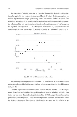
Fig. 2.7 Pareto Frontier obtained with the G-MOGA algorithm
The Pareto Frontier obtained with the G-MOGA (Figure 2.7) is a section of the original
Pareto Frontier of Figure 2.3, whose solutions are characterized by low cost and exposure
time values. Note that the ranges of these two latter objectives are significantly reduced
([402.98, 497.06] and [20.74, 25.651], respectively), while the range of the system mean
availability ([0.9986, 0.996]) is approximately the same; this is due to the lower importance
given to the system availability objective.
The Pareto Frontier is dense (still made of 100 solutions) but concentrated in the pre-
ferred region of the objective functions space: this means that the algorithm is capable of
finding a number of solutions which are preferred according to the DM requirements. This
increases the efficiency of the solutions offered to the DM but the decision problem is still
difficult because the DM has to choose between very close preferred solutions.

18. 40 Computational Intelligence Systems in Industrial Engineering
The procedure of solution reduction by clustering illustrated in Section 2.3.1.1 could,
then, be applied to the concentrated, preferred Pareto Frontier. In this case, given the
narrow objective values ranges, particularly for the cost and the worker’s exposure time
objectives, it may be difficult to assign preferences on the objectives values. For this reason,
the selection of the best representative solution is performed in absence of preferences on
the objectives values (Section 2.3.1.1). The optimal cluster radius (ra ) which maximizes the
global silhouette value is equal to 0.32, which corresponds to a number of clusters K = 5.
Fig. 2.8 GS for different cluster radius values
The resulting cluster representative solutions, i.e., the solutions in each cluster closest
to the optimal point, ideal with respect to all the objectives are showed by Level Diagrams
in Figure 2.9.
Given the regular and concentrated Pareto Frontier obtained with the G-MOGA algo-
rithm, the optimal number of clusters, and thus of representative solutions, is smaller than
in the previous case; the combined application of the G-MOGA algorithm and clustering
procedure is found to provide a small number of preferred solutions, which make it easier
for the DM to choose the final solution: the clustering procedure is really effective in re-

19. A Comparison of Methods For Selecting Preferred Solutions in Multiobjective Decision Making 41
Fig. 2.9 Level Diagrams representation of the family representative solutions closest to the ideal
solution optimizing all objectives
ducing the number of solutions to be presented to the DM, overcoming the problem of the
crowded Pareto Frontier made of close solutions in the preferred region of the domain.
On the other hand, to compute the asp coefficients to introduce DM’s reasonable trade-
offs, one has to know the expressions of the objective functions as implemented in the
search algorithm, since, for computational reasons, these expressions might be different
from those of the problem statement, e.g., to enhance the procedure of maximization or
minimization. Then, if the DM is not satisfied with the resulting Pareto Frontier, he or
she has to modify the input parameters of the genetic algorithm. These requests to the
DM might be excessive in practical applications because, as showed before, to compute
the trade-offs coefficients the DM must, at least, know the orders of magnitude of the
objectives. Without any reference value it would be then complicated to define the amount
of an objective that the DM accepts to give up for a unitary increase of another objective.
Moreover, this task becomes particularly burdensome for problems with more than two
objectives, as the required number of trade-offs to be specified increases dramatically with
the number of objectives [18].

20. 42 Computational Intelligence Systems in Industrial Engineering
2.4 Conclusions
The results of algorithms of multiobjective optimization amount to a Pareto Set of non-
dominated solutions among which the DM has to select the preferred ones. The selection is
difficult because the set of non-dominated solutions is usually large, and the corresponding
representative Pareto Frontier in the objective function space crowded.
In the end, the application of DM preferences drives the search of the optimal solution
and can be done mainly a priori or a posteriori.
In this work, a comparison of some a priori and a posteriori methods of preference
assignment is proposed. The methods have been chosen because the authors have the depth
of experience on them necessary for a detailed comparison, here performed on a case study
concerning the optimization of the test intervals of the components of a nuclear power plant
safety system. The a priori G-MOGA method considered has been showed to lead to a
focalized Pareto Frontier, since the DM preferences are embedded in the genetic algorithm
to bias the search for non-dominated solutions towards the preferred region; the a posteriori
methods considered, on the other hand, have been showed effective in reducing the number
of solutions on the Pareto Frontier.
From the results of the comparative analysis, it turns out that the a priori and a posteriori
approaches considered are not necessarily in contrast but can be combined to obtain a
reduced number of optimal solutions focalized in a preferred region, to be presented to the
DM for the decision.
However, the implementation of the a priori method seems more complicated because it
requires the assignment of preference trade-offs on the objectives values; this latter task is
difficult if the DM has no experience on the specific multiobjective problem, and the com-
plexity increases with the number of the objectives. In these cases, a posteriori procedures
can be applied alone, still with satisfactory results. In particular, the two-steps clustering
procedure introduced by the authors for identifying a small number of representative solu-
tions to be presented to the DM for the decision, has been showed to be an effective tool
which can be applied in different decision situations independently of the Pareto Frontier
size and the number of objective functions.
Bibliography
[1] ATKOSoft, Survey of Visualization Methods and Software Tools, (1997).
[2] X. Blasco, J.M. Herrero and J. Sanchis, M. Martínez, Multiobject. Optim., Inf. Sci., 178, 3908–
3924 (2008).

21. Bibliography 43
[3] J. Branke, T. Kaubler, and H. Schmeck, Adv. Eng. Software, 32, 499 (2001).
[4] J. Branke, T. Kaubler, and H. Schmeck, Tech. Rep. TR no.399, Institute AIFB, University of
Karlsruhe, Germany (2000).
[5] S. Chiu, J. of Intell. & Fuzzy Syst., 2 (3), 1240 (1994).
[6] C.A. Coello Coello, C, in 2000 Congress on Evolut. Comput. (IEEE Service Center, Piscataway
NJ, 2000), Vol. 1, p. 30.
[7] W.W. Cooper, L.M. Seiford, and K. Tone, Data Envelopment Analysis: a Comprehensive Text
with Models, Applications, References, and DEA-Solver Software (Springer, Berlin, 2006).
[8] L. Fausett, Fundamentals of Neural Networks: Architectures, Algorithms, and Applications
(Prentice-Hall, Englewood Cliffs, 1994).
[9] P. Giuggioli Busacca, M. Marseguerra, and E. Zio, Reliab. Eng. Syst. Saf., 72, 59 (2001).
[10] ICRP Publication 60, Annals of the ICRP, 21, 1 (1991).
[11] Z. Li, H. Liao, and D.W. Coit, Reliab. Eng. Syst. Saf., 94, 1585 (2009).
[12] S. Martorell, S. Carlos, A. Sanchez, and V. Serradell, Reliab. Eng. Syst. Saf., 67, 215 (2000).
[13] US Nuclear Regulatory Commission, Rates of Initiating Events at United States Nuclear Power
Plants: 1987-1995, NUREG/CR-5750 (1999).
[14] L. Rachmawati and D. Srinivasan, in Congress on Evolut. Comput., 2006 (IEEE Conference
Pubblications, 2006), p. 962–968.
[15] P.J. Rousseeuw, J. Comput. Appl. Math., 20, 53 (1987).
[16] P. Rousseeuw, E. Trauwaert, and L. Kaufman, Belgian J. of Oper. Res., Stat. and Comput. Sci.,
29 (3), 35 (1989).
[17] J.E. Yang, M.J. Hwang, T.Y. Sung, and Y. Jin, Reliab. Eng. Syst. Saf., 65, 229 (1999).
[18] E. Zio, P. Baraldi, and N. Pedroni, Reliab. Eng. Syst. Saf., 94, 432 (2009).
[19] E. Zio and R. Bazzo, Submitted to Inf. Sci. (2009).
[20] E. Zio and R. Bazzo, Eur. J. of Oper. Res., 210 (3), 624 (2011).

22. http://www.springer.com/978-94-91216-76-3