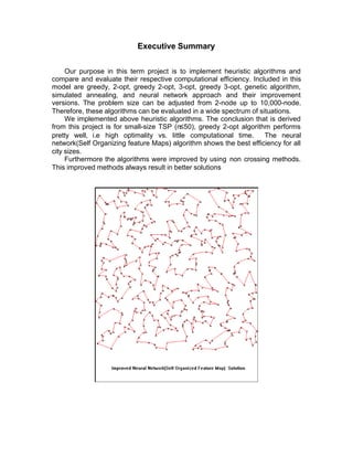
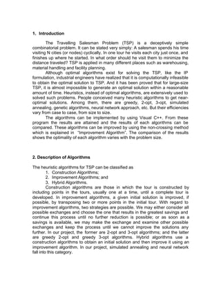
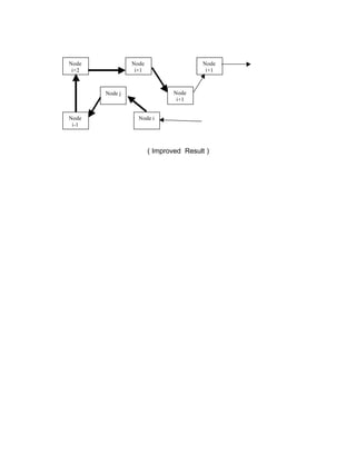
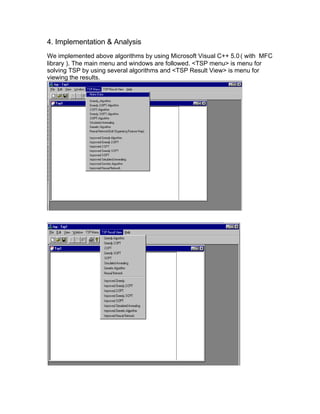
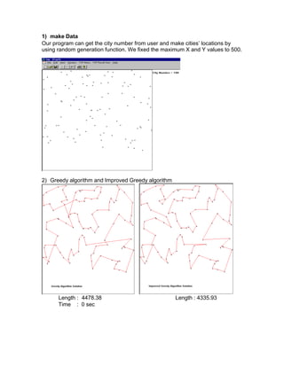
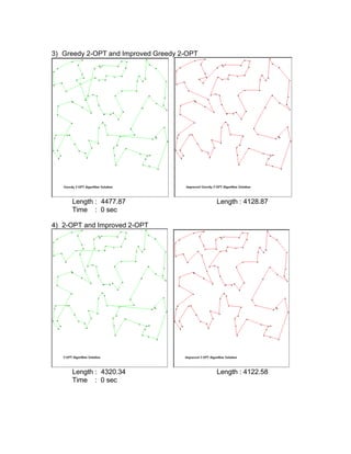
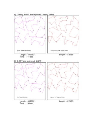
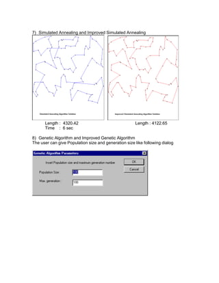
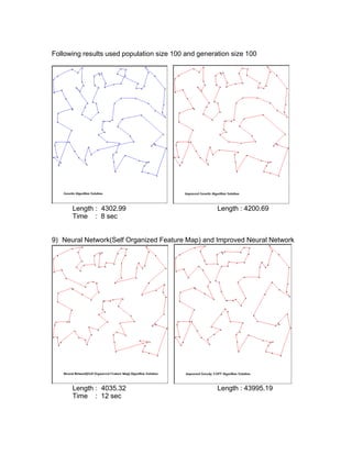
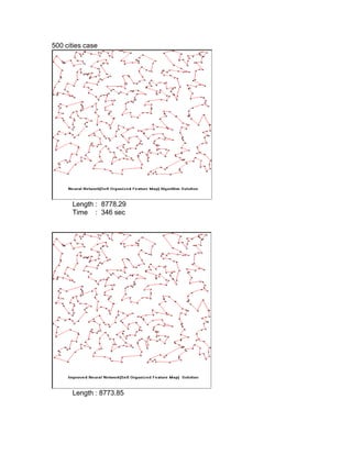
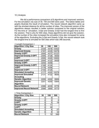
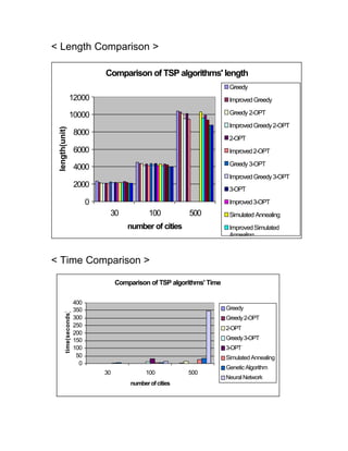
The document compares different heuristic algorithms for solving the traveling salesman problem (TSP), including greedy, 2-opt, 3-opt, genetic algorithm, simulated annealing, and neural networks. It implemented these algorithms and evaluated their computational efficiency on TSP problems of varying sizes (2-10,000 nodes). For small TSP problems (n<=50 nodes), the greedy 2-opt algorithm performed well with a high solution quality and short computation time. The neural network approach showed the best efficiency across all problem sizes. The algorithms were also improved using non-crossing methods, which always resulted in better solutions.

1. Comparison of TSP Algorithms
Project for
Models in Facilities Planning and
Materials Handling
December 1998
Participants:
Byung-In Kim
Jae-Ik Shim
Min Zhang

2. Executive Summary
Our purpose in this term project is to implement heuristic algorithms and
compare and evaluate their respective computational efficiency. Included in this
model are greedy, 2-opt, greedy 2-opt, 3-opt, greedy 3-opt, genetic algorithm,
simulated annealing, and neural network approach and their improvement
versions. The problem size can be adjusted from 2-node up to 10,000-node.
Therefore, these algorithms can be evaluated in a wide spectrum of situations.
We implemented above heuristic algorithms. The conclusion that is derived
from this project is for small-size TSP (n≤50), greedy 2-opt algorithm performs
pretty well, i.e high optimality vs. little computational time. The neural
network(Self Organizing feature Maps) algorithm shows the best efficiency for all
city sizes.
Furthermore the algorithms were improved by using non crossing methods.
This improved methods always result in better solutions

3. Table of Content
1. Introduction
2. Description of Algorithms
A. Greedy
B. 2-Opt
C. Greedy 2-Opt
D. 3-Opt
E. Greedy 3-Opt
F. Genetic
G. Simulated Annealing
H. Neural Network
3. Improvement of Algorithms
4. Simulation Results and Analysis
5. Conclusion
6. Reference
Appendix (Programming Code)

4. 1. Introduction
The Travelling Salesman Problem (TSP) is a deceptively simple
combinatorial problem. It can be stated very simply: A salesman spends his time
visiting N cities (or nodes) cyclically. In one tour he visits each city just once, and
finishes up where he started. In what order should he visit them to minimize the
distance traveled? TSP is applied in many different places such as warehousing,
material handling and facility planning.
Although optimal algorithms exist for solving the TSP, like the IP
formulation, industrial engineers have realized that it is computationally infeasible
to obtain the optimal solution to TSP. And it has been proved that for large-size
TSP, it is almost impossible to generate an optimal solution within a reasonable
amount of time. Heuristics, instead of optimal algorithms, are extensively used to
solved such problems. People conceived many heuristic algorithms to get near-
optimal solutions. Among them, there are greedy, 2-opt, 3-opt, simulated
annealing, genetic algorithms, neural network approach, etc. But their efficiencies
vary from case to case, from size to size.
The algorithms can be implemented by using Visual C++. From these
program the results are attained and the results of each algorithms can be
compared. These algorithms can be improved by using the non-crossing method
which is explained in “Improvement Algorithm”. The comparison of the results
shows the optimality of each algorithm varies with the problem size.
2. Description of Algorithms
The heuristic algorithms for TSP can be classified as
1. Construction Algorithms;
2. Improvement Algorithms; and
3. Hybrid Algorithms.
Construction algorithms are those in which the tour is constructed by
including points in the tours, usually one at a time, until a complete tour is
developed. In improvement algorithms, a given initial solution is improved, if
possible, by transposing two or more points in the initial tour. With regard to
improvement algorithms, two strategies are possible. We may either consider all
possible exchanges and choose the one that results in the greatest savings and
continue this process until no further reduction is possible; or as soon as a
savings is available, we may make the exchange and examine other possible
exchanges and keep the process until we cannot improve the solutions any
further. In our project, the former are 2-opt and 3-opt algorithms; and the latter
are greedy 2-opt and greedy 3-opt algorithms. Hybrid algorithms use a
construction algorithms to obtain an initial solution and then improve it using an
improvement algorithm. In our project, simulated annealing and neural network
fall into this category.

5. A. Greedy Algorithm
Greedy algorithm is the simplest improvement algorithm. It starts with the
departure Node 1. Then the algorithm calculates all the distances to other n-1
nodes. Go to the next closest node. Take the current node as the departing
node, and select the next nearest node from the remaining n-2 nodes. The
process continues until all the nodes are visited once and only once then back to
Node 1. When the algorithm is terminated, the sequence is returned as the best
tour; and its associated OFV is the final solution. The advantage of this algorithm
is its simplicity to understand and implement. Sometime, it may lead to a very
good solution when the problem size is small. Also, because this algorithm does
not entail any exchange of nodes, it saves considerably much computational
time.
For the C++ code for greedy algorithm, please refer to the Appendix.
B. 2-Opt Algorithm
For n nodes in the TSP problem, the 2-Opt algorithm consists of three
steps:
Step 1 Let S be the initial solution provided by the user and z its objective
function value (In our model, we use greedy algorithm to setup the initial solution
and objective function value.). Set S*=s, z*=z, i=1 and j=i+1=2.
Step 2 Consider the exchange results in a solution S’ that has OFV z’<z*,
set z*=z’ and S*=S’. If j<n repeat step 2; otherwise set i=i+1 and j=i+1. If i<n,
repeat step 2; otherwise go to step 3.
Step 3 If S≠S*, set S=S*, z=z*, i=1, j=i+1=2 and go to step 2. Otherwise,
output S* as the best solution and terminate the process.
Observe that the 2-opt algorithm considers only pairwise exchange.
Initially, the algorithm considers transposition of Nodes 1 and 2. If the resulting
solution’s OFV is smaller than that of the initial solution, it is stored as a
candidate for future consideration. If not, it is discarded and the algorithm
considers transposing of Nodes 1 and 3. If this exchange generates a better
solution, it is stored as a candidate for future consideration; if not, it is discarded.
Thus, whenever a better solution is found, the algorithm discards the previous
best solution. This procedure continues until all the pairwise exchanges are
considered. Because each node can be exchanged with n-1 other nodes and
there are n nodes in total, there are n(n-1)/2 different exchanges. These n(n-1)/2
exchanges are considered in step 2. The solution retained at the end of step 2 is
the one that provides the most improvement in the OFV. Starting with this as the
new solution, the algorithm repeats step 2 to find another better solution. At some
stage, no improvement in the current best solution is possible, and then the
algorithm terminates. The remaining solution is returned to the user as the best
one.
For the C++ code for 2-opt algorithm, please refer to the Appendix.

6. C. Greedy 2-Opt Algorithm
The greedy 2-Opt algorithm is a variant of 2-opt algorithm. It also consists
of three steps:
Step 1 Let S be the initial solution provided by the user and z its objective
function value (In our model, we use greedy algorithm to setup the initial solution
and objective function value.). Set S*=s, z*=z, i=1 and j=i+1=2.
Step 2 Transpose Node i and Node j, i<j. Compare the resulting OFV z
with z*. If z ≥ z* and j<n, set j=j+1 and repeat step 2; Otherwise go to step 3.
Step 3 If z<z*, set S*=S, z*=z, i=1, j=i+1=2 and go to step 2. If z ≥ z* and
j=n, set i=i+1, j=j+1 and repeat step 2. Otherwise, output S* as the best solution
and terminate the process.
Like the 2-Opt algorithm, greedy 2-opt algorithm also considers pairwise
exchanges. Initially, it considers transposing Nodes 1 and 2. If the resulting OFV
is less than the previous one, two nodes are immediately transposed. If not, the
algorithm will go on to Node 3 and evaluate the exchange, and so on until find
the improvement. If Nodes 1 and 2 are transposed, the algorithm will take it as an
initial solution and repeat the algorithm until it is impossible to improve the
solution any further. Greedy 2-opt algorithm makes the exchange permanent
whenever an improvement is found and thus consumes less computational time
than 2-Opt algorithm. On the other hand, greedy 2-opt produces slightly worse
solutions than 2-Opt algorithm.
For the C++ code for greedy 2-opt algorithm, please refer to the Appendix.
D. 3-Opt Algorithm
The 3-Opt algorithm is similar to the 2-opt algorithm except that it
considers transposing two nodes at a time. There are two possible ways of
transposition.: i->j->k->i
and j->k->i->j. Let’s just consider the first transposition. The steps involved are
Step 1. Let S be the initial solution and z its OFV. Set
S*=S,z*=z,i=1,j=i+1 and k=j+1.
Step 2. Consider transposing Nodes i, j, k in “i->j->k->i” fashion. If the
resulting solution S’ has a smaller z’<z*, set z*=z’ and S*=S’. If k<n, set k=k+1.
Otherwise, set j=j+1. If j<n-1, set k=j+1. Otherwise, set i=i+1, j=j+1 and k=j+1. If
i<n-2, repeat step 2. Otherwise go to step 3.
Step 3 If S≠S*, set S=S*, z=z*, i=1, j=i+1,k=j+1 and go to step 2.
Otherwise, output S* as the best solution and terminate the process.
For the C++ code for 3-Opt algorithm, please refer to the Appendix.
E. Greedy 3-Opt Algorithm
Like the greedy 2-opt algorithm, greedy 3-opt algorithm also makes the 3-
node exchange permanent whenever its resulting OFV is better than the current

7. OFV and repeats the algorithm with the new transposition as the initial solution.
Let’s just consider the “i->j->k->i” transposition again. The steps involved are:
Step 1 Let S be the initial solution provided by the user and z its objective
function value (In our model, we use greedy algorithm to setup the initial solution
and objective function value.). Set S*=S,z*=z,i=1,j=i+1 and k=j+1.
Step 2. Consider transposing Nodes i, j, k in “i->j->k->i” fashion. If the
resulting solution S’ has a smaller z’<z*, set z*=z’ and S*=S’. If k<n, set k=k+1.
Otherwise, set j=j+1. If j<n-1, set k=j+1. Otherwise, set i=i+1, j=j+1 and k=j+1. If
i<n-2, repeat step 2. Otherwise go to step 3.
Step 3 If z<z*, set S*=S, z*=z, i=1, j=i+1=2, k=j+1 and go to step 2. If z ≥ z*
and k=n, set i=i+1, j=j+1, and repeat step 2. . If z ≥ z* and j=n-1, set i=i+1, and
repeat step 2. Otherwise, output S* as the best solution and terminate the
process
The advantage of greedy 3-Opt algorithm over 3-Opt algorithm is once
again less computational time due to its less thorough search in the network.
For the C++ code for greedy 3-Opt algorithm, please refer to the
Appendix.
F. Genetic Algorithm
As the name implies, this algorithm gets its idea from genetics. The
algorithm works this way.
Step 0 Obtain the maximum number of individuals in the population P and
the maximum number of generations G from the user, generate P solutions for
the first generation’s population randomly, and represent each solution as a
string. Set generation counter Ngen=1.
Step 1 Determine the fitness of each solution in the current generation’s
population and record the string that has the best fitness.
Step 2 Generate solutions for the next generation’s population as follows:
1. Retain 0.1P of the solutions with the best fitness in the previous
population.
2. Generate 0.89P solutions via mating, and
3. Select 0.01P solutions from the previous population randomly and
mutate them.
Step 3 Update Ngen= Ngen+1. If Ngen≤G, go to Step 1. Otherwise stop.
In our project, we used the two-point crossover method, given two parent
chromosomes {x1,x2,….xn} and {y1,y2,…,yn}, two integers r and s are randomly
selected, such that 1 ≤ r ≤ s ≤ n. And the genes in positions r to s of one parent
are swapped with those of the other to get two offsprings as follows.
{x1, x2,…, xr-1, yr, yr+1,…, ys, xs+1, xs+2,…, xn}
{y1, y2,…, yr-1, xr, xr+1,…, xs, ys+1, ys+2,…, yn}
Either both or the better of the two offspring is then included in the new
population. This mutation procedure is repeated until the required number of
offspring is generated. To avoid generating infeasible solutions, we also used the

8. partially matched crossover method. Set t=r, and swaps genes xt and yt if xt≠yt in
the first parent x={x1, x2,…, xr-1, xr, xr+1,…, xs, xs+1, xs+2,…, xn}. This swapping is
done for t=r through s, one by one, and then we have a feasible offspring. The
same is done for y={y1, y2,…, yr-1, yr, yr+1,…, ys, ys+1, ys+2,…, yn}. Because the
partially matched crossover method always swaps genes within a parent,
feasible offspring are obtained.
Therefore, our model uses mutation to generate a population by swapping
any two randomly selected genes.
For the C++ code for genetic algorithm, please refer to the Appendix.
H. Simulated Annealing
The basic idea of simulated annealing(SA) is from the statistical
mechanics and is motivated by an analogy of behavior of physical systems in the
presents of a heat bath. This algorithm obtains better final solutions by gradually
going from one solution to the next. The main difference of SA from the 2-opt or
3-opt algorithm is that the local optimization algorithm is often restrict their search
for the optimal solution in a downhill direction which mean that the initial solution
is changed only if it results in a decrease in the OFV. The temperature refers to
the state through which the simulated annealing algorithm passes in its search
for a better solution. Starting with an initial temperature, we move to the next
temperature only when we have reached a frozen state. When a frozen state is
reached, the temperature is reduced by a cooling factor r, and the procedure is
repeated until a certain predetermined number of temperature steps have been
performed.
Step 0 Set S = initial feasible solution
z = corresponding OFV
T = initial temperature = 1; r = cooling factor = 0.9
ITEMP = number of times the temperature T is decreased = 0
NLIMIT = maximum number of new solutions to be accepted at
each temperature = 10n
NOVER = maximum number of solutions evaluated at each
temperature = 100n
Step 1 Repeat step 2 NOVER times or until the number of successful new
solutions is equal to NLIMIT
Step2 Pick a pair of machines randomly and exchange their positions. If the
exchange of the position of the two machines results in the overlapping of
some other pairs of cities, appropriately modify the coordinates of the
center of the concerned machines to ensure no overlapping. If the
resulting solution S* has OFV <= z, set S* = S and z = corresponding
OFV. Otherwise, compute delta = difference between z and the OFV of
the solution S*. and set S*=S with a probability e-delta/T
.
Step 3 Set T = rT and ITEMP = ITEMP + 1. If ITEMP <= 100, go to step 1;
otherwise stop.

9. For the C++ code for simulated annealing algorithm, please refer to the
Appendix.
G. Neural Network(Self Organizing Feature Maps)
First, randomly pick up any city in the network as the initial loop. The
number of nodes N on the loop grows subsequently according to a node creation
process. (see below). At each processing step, a city i is surveyed. One complete
iteration takes M (number of total cities to be visited) sequential steps, for i=1 to
i=M, thus picking every city once in a preset order. A gain parameter is used
which decreases between two complete iterations. Several iterations are needed
to go from the high gain value to the low one giving the final result.
Surveying the city i comprises the following steps:
Step 1. Find the node jc which is closed to city i.
Step 2. Move node jc and its neighbors on the ring towards city i.
The distance each node will move is determined by a function f(G,n) where G is
the gain parameter (its initial is set 10 in our model), and n is the distance
measured along the loop between nodes j and jc.
n=inf (j- jc (mod N), jc -j(mod N))
Every node j is moved from current position to a new one.
The function f is defined to be
f(G,n)=sqrt(1/2)*exp(-n2
/G2
)
This means:
- when G →∞, all nodes move towards city I with the same strength sqrt(1/2).
- when G → 0, only node jc moves towards city i.
Decreasing the gain at the end of a complete survey is done by G←(1-
α)G. α is the only parameter that has to be adjusted. It is directly related to the
number of complete surveys needed to attain the result, and hence its quality.
The gain is decreased from a high initial Gi which ensures large moves for
all nodes at each iteration step to a sufficiently low Gf for which the network is
stabilized. The total number of iterations can be computed from these two fixed
values depending only on M.
A node is duplicated, if it is chosen as the winner for two different cities in
the same complete survey. The newly created node is inserted into the ring as a
neighbor of the winner, and with the same coordinates in the plane. Both the
winner and the created node are inhibited. If chose by a city, an inhibited node
will induce no movement at all in the network for this city presentation. It is re-
enabled on the next presentation. This guarantees that the “twin nodes” will be
separated by the moves of their neighbors, before being “caught” by cities. The
maximum number of nodes created on the loop experimentally appears to be
less than 2M.
A node is deleted, if it has not been chosen as the winner by any city
during three complete surveys. This creation-deletion mechanism has proved
important to the attainment of near-optimum solutions.
For the C++ code for neural network approach, please refer to the
Appendix.

10. 3. Improvement of Algorithms
In the initial implementation of these 8 algorithms, it is found that these
algorithms do not eliminate the crossing of routes. Of course, these crossings of
routes lengthen the total distance of travel in TSP. We improved these algorithms
by getting rid of these crossings.
The process is as follows.
First, obtain the solution with any of the preceding algorithms. Second,
pick up the segment between Node 1 and Node 2, check any other segment
against the 1-2 segment to see if these 2 segments intersect each other. If not,
pick up the segment 2-3, and check consequent segment against segment 2-3. If
the intersection is found for any two distinct segments, re-route the loop. And the
process is continued sequentially throughout the network.
The mathematical implementation of both checking and re-routing is as
follows: The current 2 segments are i→i+1, j→j+1 (1 ≤ i < i+1 < j< j+1 ≤ n). The
line of i→i+1 segment can be expressed as x=xi+(xi-1 - xi)*t, y= yi +(yi+1 - yi)*t, and
the line of j→j+1 segment can be expressed as x=xj+(xj-1 - xj)*s, y= yj +(yj+1 -
yj)*s. Given these parametric expressions and the coordinates of these 4 nodes,
the coordinates and associated s, and t can be calculated for the intersection of
these lines. If both s and t are
0 ≤ t ≤ 1 and 0 ≤ s ≤ 1, it is determined that these two segments are intersected.
Otherwise not. When they are intersected, transpose node i+1 and node j. There
would be neither intersection on these 2 segments nor break of the loop.
Since there are N+1 routes for N cities, N(N+1)/2 crossing-checks are
necessary. Our model finds these non-crossing methods substantially improved
upon these algorithms for large-size problem.
( Original Result )
Node
j+1
Node j
Node i
Node
i+1
Node
j+1
Node
i+2
Node
j-1

11. ( Improved Result )
Node
j+1
Node j
Node i
Node
i+1
Node
j+1
Node
i+2
Node
j-1

12. 4. Implementation & Analysis
We implemented above algorithms by using Microsoft Visual C++ 5.0( with MFC
library ). The main menu and windows are followed. <TSP menu> is menu for
solving TSP by using several algorithms and <TSP Result View> is menu for
viewing the results.

13. 1) make Data
Our program can get the city number from user and make cities’ locations by
using random generation function. We fixed the maximum X and Y values to 500.
2) Greedy algorithm and Improved Greedy algorithm
Length : 4478.38 Length : 4335.93
Time : 0 sec

14. 3) Greedy 2-OPT and Improved Greedy 2-OPT
Length : 4477.87 Length : 4128.87
Time : 0 sec
4) 2-OPT and Improved 2-OPT
Length : 4320.34 Length : 4122.58
Time : 0 sec

15. 5) Greedy 3-OPT and Improved Greedy 3-OPT
Length : 4356.92 Length : 4124.95
Time : 11 sec
6) 3-OPT and Improved 3-OPT
Length : 4356.92 Length : 4124.95
Time : 30 sec

16. 7) Simulated Annealing and Improved Simulated Annealing
Length : 4320.42 Length : 4122.65
Time : 6 sec
8) Genetic Algorithm and Improved Genetic Algorithm
The user can give Population size and generation size like following dialog

17. Following results used population size 100 and generation size 100
Length : 4302.99 Length : 4200.69
Time : 8 sec
9) Neural Network(Self Organized Feature Map) and Improved Neural Network
Length : 4035.32 Length : 43995.19
Time : 12 sec

18. 500 cities case
Length : 8778.29
Time : 346 sec
Length : 8773.85

19. 10 ) Analysis
We did a performance comparison of 8 algorithms and improved versions.
For the simulation city size of 30, 100 and 500 were used. The below tables and
graphs illustrate the result of simulation. The neural network algorithm came up
with the shortest distance for all the number of cities. The improved version of the
algorithms always resulted in better solution compared to the original solution.
For the time of simulation, 3-Opt and Greedy 3-Opt had the longest time to find
the solution. That is why for 500 cities, these algorithms did not give the solution.
As the number of the cites increased the simulation time also increased for some
of the algorithms. Excluding the 3-Opt and Greedy 3-Opt, the neural network took
the longest time to simulate for 500 cites which was 346 seconds.
< Length Comparison >
Algorithm City Size 30 100 500
Greedy 2330 4478 10402
Improved Greedy 2187 4335 10279
Greedy 2-OPT 2095 4377 10127
Improved Greedy 2-OPT 2095 4128 9500
2-OPT 2095 4320 10083
Improved 2-OPT 2095 4122 9459
Greedy 3-OPT 2240 4356
Improved Greedy 3-OPT 2168 4124
3-OPT 2178 4356
Improved 3-OPT 2155 4124
Simulated Annealing 2177 4320 10279
Improved Simulated
Annealing
2131 4122 9606
Genetic Algorithm 2295 4302 9906
Improved Genetic
Algorithm
2201 4200 9364
Neural Network 2086 4035 8778
Improved Neural Network 2086 3995 8773
< Time Comparison >
Algorithm City Size 30 100 500
Greedy 0 0 1
Greedy 2-OPT 0 0 2
2-OPT 0 0 14
Greedy 3-OPT 0 11
3-OPT 0 30
Simulated Annealing 2 6 27
Genetic Algorithm 6 8 34
Neural Network 1 12 346

20. < Length Comparison >
< Time Comparison >
Comparison of TSP algorithms' length
0
2000
4000
6000
8000
10000
12000
30 100 500
number of cities
length(unit)
Greedy
ImprovedGreedy
Greedy 2-OPT
ImprovedGreedy2-OPT
2-OPT
Improved2-OPT
Greedy 3-OPT
ImprovedGreedy3-OPT
3-OPT
Improved3-OPT
Simulated Annealing
ImprovedSimulated
Annealing
Comparison of TSP algorithms' Time
0
50
100
150
200
250
300
350
400
30 100 500
numberofcities
time(seconds)
Greedy
Greedy2-OPT
2-OPT
Greedy3-OPT
3-OPT
Simulated Annealing
Genetic Algorithm
Neural Network

21. 5. Conclusion
We implemented the above-mentioned heuristic algorithms. It is shown that
the algorithms were improved by using non crossing methods. This improved
methods always result in better solutions. The conclusion that is derived from this
project is for small-size TSP (n≤50), greedy 2-opt algorithm performs pretty well,
i.e high optimality vs. little computational time. The neural network(Self
Organizing feature Maps) algorithm demonstrates the best efficiency for all city
sizes. Through the simulation, the improved neural network algorithm gives us
the shortest distance for 30 cities, 100 cities and 500cities. The number of the
cities doesn’t affect the optimality of algorithms. Therefore no matter how many
cities are involved in the Travelling salesman problem, the Neural network
algorithm will give the best solution of all these 16 algorithms that were
mentioned in this report. The simulation of 3-Opt algorithm take a very long time
for a large number of cities such as 500. It is not efficient to use 3-Opt algorithm
for problem with more than 100 cites.
For small-size TSP (n≤50), improved greedy 2-opt algorithm is
recommended. For medium-size TSP (50≤n≤100), improved 2-opt algorithm and
neural network are recommended for their optimality and efficiency. For large-
size problem (100≤n≤500), the improved genetic algorithm is recommended. For
any problem-size, if the computational time is not a constraint, the improved
neural network is always recommended.
6. References
Angeniol, B., Vaubois, G de L C. and Texier JYL.(1988) Self-Organizing Feature
Maps and the Traveling Salesman Problem, Neural Networks, Vol 1, pp 289-293.
Heragu, Sunderesh (1997) Facilities Design, PWS Publishing Company, Boston,
MA.