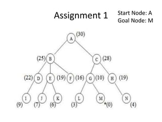
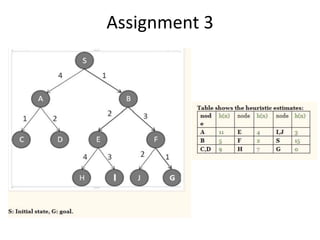
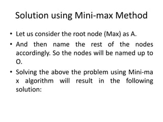
Download to read offline

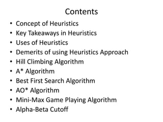

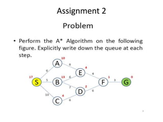
![Solution
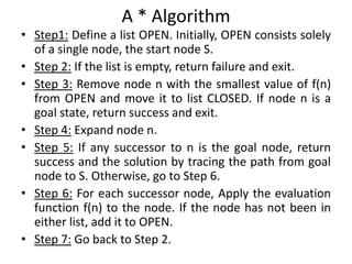
• Initialization: Close List [], Open List []
• Step 1:
• Open List [S]
• Closed List []
• Step2:
• Open List [B, A]
• Closed List [S]
• Step 3:
• Open List [F, E, A]
• Closed List [S, B]
• Step 4:
• Open List [G, E, I, A]
• Closed List [S, B, F]
• Step 5:
• Open List [E, I, A]
• Closed List [S, B, F, G] So backtrack to Source Node.
Start Node: S
Goal Node: G
Solution Path: S>B>F>G](https://image.slidesharecdn.com/heuristicsearchingalgorithms-240109233311-8a762fcc/85/Heuristic-Searching-Algorithms-Artificial-Intelligence-pptx-32-320.jpg)
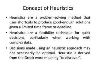
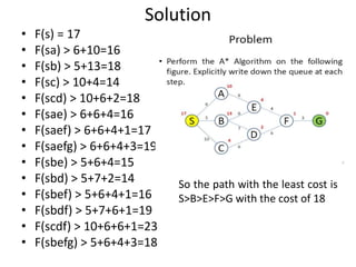
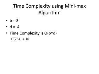
![Solution
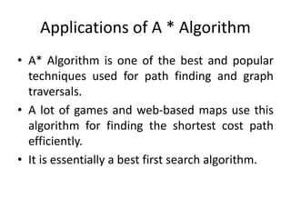
• Initialization: Open[], Closed[]
• Step 1
• Open[A]
• Closed[]
• Step 2:
• Open[D, B, C]
• Closed[A]
• Step 3:
• Open[E, B, C, F]
• Closed[A, D]
• Step 4:
• Open[J, B, C, F, I]
• Closed[A, D, E]
• Step 5:
• Open[B, C, F, I]
• Closed[A, D, E, J]
• Path: A>D>E>J](https://image.slidesharecdn.com/heuristicsearchingalgorithms-240109233311-8a762fcc/85/Heuristic-Searching-Algorithms-Artificial-Intelligence-pptx-37-320.jpg)


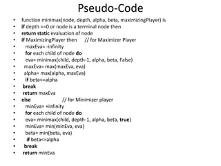
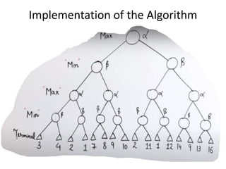

The document discusses various heuristic search algorithms used in artificial intelligence including hill climbing, A*, best first search, and mini-max algorithms. It provides descriptions of each algorithm, including concepts, implementations, examples, and applications. Key points covered include how hill climbing searches for better states, how A* uses a cost function to find optimal paths, and how best first search uses a priority queue to search nodes in order of estimated cost to reach the goal.