Commutative algebra

Some Applications of Commutative Algebra
to String Theory

Paul S. Aspinwall

1 Introduction

String theory was first introduced as a model for strong nuclear interactions, then
reinterpreted as a model for quantum gravity, and then all fundamental physics.
However, one might argue that its most successful applications to date have
been in the realm of pure mathematics and geometry. The superstring is most
easily understood in ten dimensions. In order to make contact with the observed
physical world of four spacetime dimensions, one compactifies on a six-dimensional
manifold. This is most easily analyzed in the case where this manifold is a Calabi–
Yau threefold. Fortuitously, such varieties happen to be of great mathematical
interest.
Historically, geometry, as used by physicists, has generally been differential
geometry because of its role in general relativity. More recently, especially because
of the use of supersymmetry, string theory has come to rely more heavily on
algebraic geometry. Thus tools in commutative algebra have become more useful
in recent years. A simplified model of great interest in string theory, known as
topological field theory, is where the connections to commutative algebra become
most manifest.
The purpose of this chapter is to review some particular applications of commu-
tative algebra to string theory. Developments in recent years in computer packages
for commutative algebra, such as Macaulay 2 [1], mean that it is of great practical
value if a problem can be translated into a question in commutative algebra. We will
discuss three examples where this happens.
The first two applications are closely related and involve the structure of
topological field theory itself. Certain products in the theory can be interpreted as

P.S. Aspinwall ( )
Mathematics Department, Duke University
e-mail: psa@cgtp.duke.edu

I. Peeva (ed.), Commutative Algebra: Expository Papers Dedicated to David Eisenbud 25
on the Occasion of His 65th Birthday, DOI 10.1007/978-1-4614-5292-8 2,
© Springer Science+Business Media New York 2013

26 P.S. Aspinwall

Ext computations for sheaves on the Calabi–Yau or in terms of matrix factorizations
that are very amenable to computer algebra. This may also be viewed intrinsically as
an efficient way to compute certain Ext groups. As a by-product, we are also able to
see some elements of Hochschild cohomology that are relevant for open-to-closed
string transitions.
The final application is related to monodromy. This can be viewed as monodromy
of integral 3-cycles in a Calabi–Yau threefold under loops in the moduli space
of complex structures or, via mirror symmetry, as automorphisms of the derived
category induced by varying the complexified K¨ hler form. This monodromy is
a
also related to solutions of the well-studied GKZ system of differential equations.
We show how this monodromy can be stated in terms of a ring which we compute
in a fairly nontrivial example.

2 Categorical Topological Field Theory

2.1 Closed String Theories

Before we look at the applications, we will review a contemporary mathematical
picture of string theory. As a string moves through space and time, it sweeps
out a surface known as the worldsheet. A central idea in string theory is that
one “pulls back” physics from spacetime to the worldsheet, thus reducing physics
problems to problems in two-dimensional field theory. Of particular interest are field
theories on the worldsheet which are invariant under two-dimensional conformal
transformations, i.e., “conformal field theories.” Some of the structure of conformal
field theories can be determined by much simpler “topological field theories.”
Fortunately, all the mess and non-rigor of quantum field theory can be avoided in
topological field theories, as they have a nice direct categorical description thanks to
Atiyah [2] based on some then-unpublished ideas by Segal. We will briefly review
this picture here, but we refer to [3], Chap. 2 in [4] and references therein for a more
complete treatment.
Let Cobc be a category whose objects are closed oriented 1-dimensional
manifolds, i.e., disjoint unions of circles. Given a pair of objects, M and N , a
morphism is a cobordism from M to N . Diffeomorphic cobordisms are considered
equivalent. Note` we preserve orientations in the sense that the boundary of a
that
cobordism is M N , where M is the orientation-reversed M .
Composing cobordisms gives an obvious category structure on Cobc , where the
identity morphism may be taken to be the cylinder M Œ0; 1. Cobc is a monoidal
category, i.e., it has a tensor product on objects and a unit object. In this case the
tensor product is disjoint union, and the unit object is empty.
Let Vect be the monoidal category of vector spaces over a field k. Here tensor
product is the usual tensor product of vector spaces and the unit object is the one-
dimensional space k.

Some Applications of Commutative Algebra to String Theory 27

Definition 1. A “closed-string topological field theory” is a functor, respecting the
monoidal structure, from Cobc to Vect.
Such theories are specified by very little data. First we specify the vector space
associated to a single circle. This is called the “Hilbert space” of the theory. Then we
need to give the morphisms of vector spaces associated to a few basic morphisms.
Then the full structure of the theory can be derived by sewing these basic morphisms
together.
Let X be a Calabi–Yau threefold. That is, X is a quasi-projective complex
algebraic variety of dimension three with trivial canonical class. We assume the
covering space of X does not have an elliptic curve factor. Usually X will be
smooth, and thus we often refer to it as a manifold. One of the richest applications
of topological field theories is to such varieties. Given such a manifold, X , there are
two associated theories—the A-model and the B-model.
The central object of study in this chapter is the B-model, which is a good deal
easier than the A-model and which we define first. The B-model is completely
algebraic in nature, although we will assume for purposes of presentation that we
always work over C. The data is:
• The Hilbert space associated to a circle is

M
3
Hı D H q .X; ^p T /; (1)
p;qD0

where T is the tangent sheaf of X . Obviously we have a bigraded structure .p; q/
here. The single grading given by p C q is instrinsic to the topological field
theory, as we discuss below. In the case that b1 .X / D 0, the topological field
theory structure factorizes into even and odd p C q. We can then consistently
restrict attention to the subspace where p D q.
• The left cap is mapped by the functor to a map k ! Hı . The image of 1 is
1 2 H 0 .X; ØX /.
• The right cap yields a map Hı ! k which is only nonzero on the degree .3; 3/
R
part of Hı . If ŒAij k 2 H 3 .X; ^3 T /, then the resulting value is X ^ N ij k Aij k ,
where is a choice of nonzero holomorphic 3-form and indices are lowered and
raised using the K¨ hler metric.
a

• gives a product Hı ˝ Hı ! Hı , which is the wedge product (extended
to exterior powers of the tangent sheaf) on Hı . Note that this wedge product
is commutative only up to a sign. This is a spin theory, the sense of Sect. 2.1.6
of [4].
This information is enough to completely determine the topological field theory. For
example, it follows that:

• gives a nondegenerate pairing Hı ˝ Hı ! k.

28 P.S. Aspinwall

P
• yields a map 1 7! i i ˝ i , where f 1 ; 2 ; : : :g is a basis for Hı , and
the i ’s are dual with respect to the above pairing.

• The torus, which is the composition , is the map k ! k given by
multiplying by the Euler characteristic .X /.
• Because of the grading, a Riemann surface of genus ¤ 1 gives 0.
The A-model depends on the symplectic geometry of X . A complexified K¨ hler a
form B C iJ 2 H 2 .X; C=Z/ is part of the basic data on which the model depends.
Here J is the usual K¨ hler form, while B 2 H 2 .X; R=Z/ represents the “B-field”
a
which is ubiquitous in string theory. The Hilbert space of closed strings is given by
the De Rham cohomology of X . The complexity of the A-model comes from the
fact that the product Hı ˝ Hı ! Hı depends on “instanton corrections” coming
from rational curves (see, e.g., [5]).

2.2 Open–Closed Strings

One obtains a much richer structure if one allows for open strings as well as closed
strings. That is, the worldsheet may have a boundary. Thus, we need a new category
Coboc whose objects are disjoint unions of oriented circles and line segments. The
morphisms are cobordisms consisting of manifolds possibly with boundaries.
The boundaries allow us to decorate the category further. Each segment of the
boundary of a cobordism and each end of a line segment object should be labeled
by a “boundary condition.” Such boundary conditions are called “D-branes.” We
consider the set of D-branes as part of the information in Coboc . A morphism in
Coboc may look something like

b
c b
b
b a
a a

where the letters represent D-branes.
Definition 2. An “open–closed-string topological field theory” specifies a partic-
ular set of D-branes and gives a functor, respecting the monoidal structure, from
Coboc to Vect.


While this definition allows for an arbitrary set of D-branes, the A-model and
B-model endow this set with a particular structure. It is key to note that such a field
theory immediately gives the set of D-branes themselves a categorical structure,
with D-branes as objects. The set of morphisms Hom.a; b/ is given by the Hilbert
space associated with the line interval going from D-brane a to D-brane b. A
composition of morphisms is given by

c c

b c
b
b a
a a
(2)

and the identity in Hom.a; a/ is the image of 1 in the map k ! Hom.a; a/ induced
by the cobordism from nothing to the line interval:

a
a
a
(3)

Furthermore, D-branes can “bind together” to form other D-branes which gives
this category a triangulated structure, but we will not use this structure in this
chapter. In the case of the B-model on a Calabi–Yau threefold X , it is widely
believed that the D-brane category is the bounded derived category of coherent
sheaves on X .1
Similarly, the D-brane category for the A-model is generally taken to be the
(derived) Fukaya category [9]. Objects in this category are (certain) Lagrangian 3-
cycles in X . Fortunately, for the purposes of this chapter, we need to know little
further about this category.
Definition 3. Two Calabi–Yau threefolds, X and Y , are said to be a “mirror pair”
if there is a natural isomorphism between the open–closed topological field theory
functors associated with the A-model on Y and the B-model on X . This implies
“homological mirror symmetry” which is an equivalence between the D-brane
categories.

1
The basic idea of a proof was proposed in [6] and further studied in [4, 7, 8]. The current physics
proofs only say that D-brane category has the derived category as a full subcategory.

30 P.S. Aspinwall

2.3 Topological Conformal Field Theory

One may obtain a further richer theory which is “almost topological” by retaining
a little more information than just the diffeomorphism class of a cobordism. Fixing
two objects M and N , let M .M; N / be the moduli space of Riemann surfaces
giving a cobordism from M to N . The category dgCoboc is defined to have the same
objects as Coboc , but now the morphisms will be geometric cochain complexes on
M .M; N /. This gives dgCoboc the structure of a dg-category. Let dgVect be the
dg-category of cochain complexes of vector spaces. A “topological conformal field
theory” (TCFT)2 is then a dg-functor from dgCoboc , together with a set of D-brane
labels, to dgVect. We refer to [11] for a full description.
Note that a Hilbert space is now a complex of vector spaces rather than a
single vector space. The original topological field theory Hilbert space can be
recovered from this simply by taking the cohomology groups of these complexes.
The homological grading naturally gives a grading to the Hilbert spaces involved.
These gradings were seen above in the A and B-models.
The dg-category structure now extends to the D-brane category too. The TCFT
associated a line interval from a to b with a chain complex of vector spaces. The ho-
mological grading on this complex can be formally extended to the
D-branes themselves by defining Hom.aŒi ; bŒj / in the category to be the complex
Hom.a; b/ shifted left j i places. This agrees with the usual translation functor
on the derived category.
In the case of the B-model on a smooth Calabi–Yau threefold, this dg structure
arises naturally from Dolbeault cohomology on vector bundles. That is, if two
D-branes are locally free sheaves E and F , the complex of morphisms between
them is given by

N
@ N
@
0 G €.A 0;0 ˝ E _ ˝ F / G €.A 0;1 ˝ E _ ˝ F / G: : : ; (4)

where A 0;q is the sheaf of C 1 .0; q/-forms and € is the global section functor. This
can then be extended in the usual way when the D-branes are complexes of locally
free sheaves.

2.4 Hochschild Cohomology

We saw above that a collection of D-brane labels and a topological field theory give
the data to construct a D-brane category. In the TCFT case the converse is also true.

2
In physics language this is phrased as coupling a topological field theory to topological gravity.
The term TCFT actually means something quite different in the physics literature [10].


That is, given a D-brane dg-category, one can completely reconstruct the TCFT.
This was proven by Costello [11], but we can give a quick idea of how this works
here. First deﬁne Á mapping a D-brane object a to a morphism Á .a/ 2 Hom.a; a/
as the image of in the Hilbert space of closed strings via the diagram:

a
φ∈ ηφ (a)
a
(5)

Now note the equivalence of the morphisms:

b b b
b a a b
b =
b a a
a a a
(6)

Let id be the identity functor from the D-brane category to itself. Rewriting (6) in
algebraic form gives a commutative diagram that states precisely that Á is a natural
transformation from id to id. Given that the D-brane category is a dg-category,
the work of [12] shows that this can be viewed as Hochschild cohomology. To be
precise, for a D-brane category B, the Hochschild cohomology is written

HH i .B/ D Nat.idB ; idB Œi /: (7)

In this way one identiﬁes the Hochschild cohomology of the D-brane category with
the Hilbert space of closed string states (complete with its homological grading)
[11].
Furthermore we can recover the “pants diagram” combining two closed strings.
This comes from the natural product rule on Hochschild cohomology coming from
combining natural transformations and can be put in diagrammatic form:

b b

b b
b = b
b a b a
a a a a
(8)
We close this section by noting that all the constructions above for the B-model
can be stated in purely algebraic terms. This is what allows us to attack the B-model
by using the tools of commutative algebra and what makes the B-model much more
amenable to study than the A-model.

32 P.S. Aspinwall

3 Toric Geometry and Phases

A versatile context in which to apply the tools of commutative algebra is to consider
compact Calabi–Yau threefolds which are complete intersections in toric varieties.
We also need to consider noncompact Calabi–Yau varieties (of dimension possibly
greater than 3) which are toric varieties themselves. We begin with the latter.
Let N be a lattice of rank d . Let P be a convex polytope in N ˝ R such that
the vertices of the convex hull lie in N . Furthermore, we demand that P lies in a
hyperplane of N ˝ R. Let A denote the set of points P N and let n denote the
number of elements of A .
The coordinates of the points of A form a d n matrix defining a map A W
Z˚n ! N which we assume is surjective. Form an exact sequence

A
0 G L G Z˚n G N G 0; (9)

where L is the “lattice of relations” of rank r D n d . Dual to this we have

ˆ
0 G M G Z˚n G D G 0; (10)

where ˆ is the r n matrix of “charges” of the points in A .
Let
S D CŒx1 ; : : : ; xn : (11)
The matrix ˆ gives an r-fold multigrading to this ring. In other words, we have a
.C /r torus action:
xi 7! ˆ1i ˆ2i : : : ˆri xi ;
1 2 r (12)
where j 2 C . Let S0 be the .C /r -invariant subalgebra of S . The algebra S then
decomposes into a sum of S0 -modules labeled by their r-fold grading:
M
SD S˛ ; (13)
˛2D

where D Š Z˚r from (10). As usual we denote a shift in grading by parentheses,
i.e., S.˛/ˇ D S˛Cˇ .
Consider a simplicial decomposition of the point set A which is regular in the
sense of [13]. This simplicial decomposition may or may not include points in the
interior of the convex hull of A . We refer to a choice of simplicial decomposition
as a “phase.”
To each phase we associate the “Cox ideal” defined in [14] as follows.
Definition 1. Let † D f 1 ; 2 ; : : :g denote the set of simplices of maximum
dimension. If is a simplex, we say i 2 if the i th element of A is a vertex
of . Then


0 1
Y Y
B† D @ xi ; xi ; : : :A : (14)
i 62 1 i 62 2

Clearly B† is a square-free monomial ideal in S .
Definition 2. Let V .B† / denote the subvariety of Cn given by B† . Then

Cn V .B† /
Z† D : (15)
.C /r

For examples of this construction we refer to Sect. 5.1 of [15]. Cox [14] shows
that there is a correspondence between finitely generated graded S -modules and
coherent sheaves on a smooth Z† which follows the usual correspondence between
sheaves and projective varieties as in Chap. II.5 of [16]. If U is an S -module, we
e e
denote U as the corresponding sheaf. U is zero as a sheaf if and only if U is killed
by some power of B† . This yields
Proposition 1. Assume Z† is a smooth toric variety. Then

Db .gr S /
Db .Z† / D ; (16)
T†

where Db .gr S / is the bounded derived category of finitely generated multigraded
S -modules and T† is the full triangulated subcategory generated by modules killed
by a power of B† . This quotient of triangulated categories is the “Verdier quotient”
(see, e.g., [17]).
Actually we can extend this proposition to the case where Z† is not smooth. A
graded S -module corresponds to a sheaf on the quotient stack Cn =.C /r . That is,
Db .gr S / is the derived category of coherent sheaves on this stack. Quotienting
by T† in (16) is equivalent to removing the pointset V .B† /. Thus we see a direct
correspondence between (15) and (16) and the above proposition remains true in
the singular case so long as we view sheaves in this quotient stack sense. Actually,
this is very natural from the physics perspective. One may construct the topological
B-model as a symplectic quotient in terms of the “gauged linear -model” [18].
D-branes can be described directly in this context [19]. It has also been argued
elsewhere [20] that stacks are the correct language for D-branes.
We now have the following statement from physics [5] which we assume, for
purposes of this chapter, to be true:
Physics Proposition 1. The B-model on X does not depend on the K¨ hler form
a
of X .
This has an immediate consequence. The K¨ hler form is associated to the
a
moment map of the symplectic quotient of the gauged linear -model, which, when
varied, can change the triangulation †. Thus, assuming the above proposition, we
have

34 P.S. Aspinwall

Proposition 2. Db .Z† / does not depend on the chosen triangulation †, i.e., it is
independent of the phase.
This is quite easy to verify directly when r (the rank of torus action) is one, as
done in [19, 21]. The combinatorics become more intricate for r > 1.
Let I† be the Alexander dual of the monomial ideal B† . I† is then the Stanley–
Reisner ideal of the triangulation † [22]. Suppose

I† D hm1 ; m2 ; : : :i; (17)

for monomials m1 ; m2 ; : : :. Then we have a primary decomposition

B† D m_ m_ : : : ;
1 2 (18)

where, if mj D x˛ xˇ x : : :, then m_ D hx˛ ; xˇ ; x ; : : :i.
j
It follows that .S=m_/.˛/ is annihilated by B† , where .˛/ is any shift in
j
multidegree. In fact these modules form the building blocks of T† as proven in [23]:
Proposition 3. T† is the smallest triangulated full subcategory of Db .gr S /
containing the objects .S=m_/.˛/. That is, T† is generated by iteratively applying
j
mapping cones between objects of the form .S=m_/.˛/Œn for any ˛ and n.
j

3.1 Tilting Collections

The derived category of an arbitrary algebraic variety can be difficult to describe in
concrete terms. However, in some cases, the description can be simplified due to the
existence of tilting objects.
A tilting sheaf T on Z† satisfies:
1. Exti † .T ; T / D 0 for all i < 0.
Z
2. A D HomZ† .T ; T / has finite global dimension.3
3. The direct summands of T generate Db .Z† /.
In this case the functors

R HomZ† .T ; / W Db .Z† / ! Db .mod-A/
L
(19)
˝A T W Db .mod-A/ ! Db .Z† /

are mutual inverses, where mod-A is the category of finitely generated right
A-modules.

3
In the context of this chapter, this condition is automatically satisfied.


In practice one can frequently, if not always, construct such a tilting sheaf as a
Q
sum of sheaves of the form S .˛/ as follows. For each m_ in (18), we can consider
j
the free resolution of the S -module S=m_:j

L L
::: G S.qi 2 / G S.qi1 / GS G S G 0: (20)
i i m_j

Sheafifying, this gives an exact sequence
L L
::: G Q
S .qi 2 / G Q
S .qi1 / GS
Q G 0; (21)
i i

Q Q
relating S to other objects in Db .Z† / composed of S .˛/’s for various multidegrees
˛. By considering such relations for all m_ ’s, one can try to find a minimal
j
Q Q Q
generating set fS.˛1 /; S .˛2 /, : : : ; S .˛k /g from which all others may be built. This
set thus generates Db .Z† /. Then, if all higher Ext’s between these sheaves vanish,

Q Q Q
T D S .˛1 / ˚ S .˛2 / ˚ : : : ˚ S .˛k / (22)

is a tilting object. Obviously one may shift all the ˛i ’s by some common multide-
gree, and T will remain a tilting sheaf.
Q Q Q
We will refer to fS.˛1 /; S .˛2 /; : : : ; S .˛k /g as a tilting collection. It is useful to
impose one further condition:
Q Q Q
Definition 6. A †-tilting collection of sheaves fS .˛1 /; S .˛2 /; : : : ; S .˛k /g is a
collection of sheaves forming a tilting object (22) and such that (using (16))

Hom Db .gr S/
Q Q
.S .˛i /; S .˛j // Š HomDb .gr S / .S.˛i /; S.˛j //; (23)
T†

for all i; j .
If T given by (22) corresponds to a †-tilting object then let Db .gr S /T be the
full triangulated subcategory of Db .gr S / generated by fS.˛1 /; S.˛2 /; : : : ; S.˛k /g.
It immediately follows that
Proposition 4. There is an equivalence of categories

Db .gr S /
Š Db .gr S /T : (24)
T†

This is easy to see given that there is an equivalence between morphisms on both
sides for objects in the tilting collection, and furthermore all objects may be built
from the tilting objects.
The conditions on a †-tilting collection can be expressed conveniently in terms
i
of local cohomology. Let HB .S / be the local cohomology groups of the monomial

36 P.S. Aspinwall

ideal B. These groups carry the same multigrading structure as S , and we denote
i
the graded parts HB .S /˛ accordingly. We then have the following copied from [24]:
Proposition 5. For i > 0 there are isomorphisms
Q
H i .Z† ; S .˛// Š HBC1 .S /˛
i
(25)

and an exact sequence
0 G S˛ G H 0 .Z† ; S .˛//
Q G H 1 .S /˛ G 0: (26)
B

This gives
Q Q Q
Proposition 6. If fS .˛1 /; S .˛2 /; : : : ; S.˛k /g forms a †-tilting collection then
i
HB .S /˛i ˛j D0 (27)

for all i 0 and all i; j .
In the case that r D 1 and we have a single grading, the process of finding a
tilting sheaf is very straightforward [19, 21, 25]. Here, one obtains simply a range
Q Q Q
T D S .a/ ˚ S .a C 1/ ˚ : : : ˚ S .a C k 1/ (28)
for any choice of a.
†-tilting collections become very useful if they are simultaneously †1 -tilting and
†2 -tilting for two phases †1 and †2 . Then one can use it to explicitly map objects
in the D-brane category between different phases. That is, we have an explicit
equivalence between two phases given by Proposition 4:

Db .Z†1 / G Db .gr S /T G Db .Z† /: (29)
2

In the case of r D 1, this idea has been explored in [19, 21, 25]. The combinatorics
of finding simultaneous tilting objects for many phases when r D 2 was discussed
in [26].

3.2 Complete Intersections

Because of Serre duality it is impossible to find a tilting collection on a compact
Calabi–Yau variety. That said, we may still make use of the above technology by
considering embedding the variety into a toric variety. Divide the homogeneous
coordinates of S into two sets by relabeling x1 ; : : : ; xn as p1 ; : : : ; ps , z1 ; : : : ; zn s .
Let S 0 D CŒz1 ; : : : ; zn s . Assume there is a .C /r -invariant polynomial, called a
superpotential, W 2 S that can be written

W D p1 f1 .z1 ; z2 ; : : :/ C p2 f2 .z1 ; z2 ; : : :/ C : : : C ps fs .z1 ; z2 ; : : :/; (30)

where f1 ; f2 ; : : : forms a regular sequence in S 0 .


Let X† Z† be the critical point set of W. If the functions fj are sufficiently
generic, the matrix of derivatives of these functions will have maximum rank. This
maximal rank condition will imply that, for suitable †, X† is a smooth complete
intersection in Z† . We are interested in the case where X† is a compact Calabi–Yau
threefold.
Now assume that the triangulation † is such that all the points corresponding to
the pj ’s are vertices of every simplex. That is, B† hpj i D 0 for j D 1; : : : ; s,
which implies B† may be viewed as an ideal of S 0 .
Define the ring
S0
AD : (31)
hf1 ; f2 ; : : : ; fs i
The category of coherent sheaves on X† is then the Serre categorical quotient
gr A
; (32)
M†
where M† is the abelian subcategory of all graded A-modules killed by some power
of B† . Thus, in analogy to (16), we have
Db .gr A/
Db .X† / D : (33)
T†
Now let us introduce the notion of the category of matrix factorizations. S has
an r-fold grading from the toric data. In addition, we add one further grading which
we call the R-grading. This grading lives in 2Z, i.e., it is always an even number.
For the superpotential (30) we may choose the variables pj to have R-degree 2 and
the zk ’s to have degree 0.
Define the category DGrS.W/ of matrix factorizations of W as follows. An
object is a pair
u1 Á
N
P D P1 o GP ; (34)
0
u0

where P0 and P1 are two finite rank graded free S -modules. The two maps satisfy
the matrix factorization condition

u0 u1 D u1 u0 D W:id; (35)
where both u0 and u1 have degree 0 with respect to the toric gradings (i.e., they
preserve the toric grading). u0 is a map of degree 2 with respect to the R-grading
while u1 has degree 0. Morphisms are defined in the obvious way up to homotopy.
We refer to [23, 27] for more details. The category DGrS.W/ is a triangulated
category with a shift functor

u0 Á
N
P Œ1 D P0 o G P f2g ; (36)
1
u1

38 P.S. Aspinwall

where fg denotes a shift in the R-grading. Thus

N N
P Œ2 D P f2g; (37)

and the R-symmetry grading is identiﬁed with the homological grading (and
extended from 2Z-valued to Z-valued). That is, there is no difference between Œm
and fmg in this category, although we will sometimes use both notations for clarity.
We now have
Proposition 7. There is an equivalence of triangulated categories:

DGrS.W/ Š Db .gr A/: (38)

This result follows very explicitly from the way that Macaulay 2 performs the
computation of Ext groups in the category of graded A-modules as explained in
detail in [28]. This algorithm was based on observations in [29, 30] as follows. An
A-module typically has an inﬁnite free resolution. In the case that s D 1 (i.e., a
hypersurface), the resolution is 2-periodic. This resolution can then be reinterpreted
as a system of maps between S 0 -modules, where the product of two maps forms
a matrix factorization as above. To extend this to the case s > 1, and in order to
correctly keep track of Ext data, one introduces new variables p1 ; : : : ; ps extending
the ring S 0 to S . We refer to [23] for more details.
It might help to view DGrS.W/ as the D-brane category on the stack X , where
X is the critical point set of W on the quotient Cn =.C /r . Anyway, we have an
equivalence of categories

DGrS.W/
Db .X† / Š : (39)
T†

This gives us an analogy between D-branes on X† and D-branes on Z† . In the
case of Z† we began with D-branes on the quotient stack Cn =.C /r in the form
Db .gr S / and then removed the pointset V .B† / by quotienting the category by T† .
Now in the case of X† the original stack D-brane category is DGrS.W/, and we
again remove the pointset V .B† / by quotienting the category by T† .
The fact that the D-brane category is of this form has a direct physics derivation
using the gauged linear -model in [19]. That is,
Physics Proposition 2. The D-brane category for the B-model on the critical point
set of the superpotential W is
DGrS.W/
: (40)
T†
Most importantly, combining this with Physics Proposition 1 gives us the following
notion:


Physics Proposition 3. The category

DGrS.W/
(41)
T†

does not depend on the choice of triangulation †.
We refer to [21] and the recent work [31] for more rigorous statements using GIT
language.
Note that the quotient in the above statement needs some interpretation. Let M
be an S -module that is annihilated by W. Then M is an S=hWi-module. A free
resolution of M as an S=hWi-module results in a matrix factorization and thus
maps M into DGrS.W/. One should therefore consider T† in (40) and (41) to be
generated by S -modules annihilated both by a power of B† and by W. Note that in
very simple examples, W 2 B† anyway, but this need not be the case generally.
As an example let us consider the following. Let the toric geometry be given by
a homogeneous coordinate ring S D CŒp; t; x0 ; x1 ; x2 ; x3 ; x4 with degrees

p t x0 x1 x2 x3 x4
Q1 4 1 1 1 1 0 0
(42)
Q2 0 20 0 0 1 1
R 2 0 0 0 0 0 0

and superpotential

W D p.x0 C x1 C x2 C t 4 x3 C t 4 x4 /:
4 4 4 8 8
(43)

There is a triangulation of the pointset that has p as a vertex of every simplex and t
is ignored completely. This gives a monomial ideal I† D hx0 x1 x2 x3 x4 ; ti and

B† D hx0 ; x1 ; x2 ; x3 ; x4 ihti: (44)

Z† then corresponds to the total space of the canonical line bundle over the
weighted projective space P4 f22211g
. One calls this the “orbifold” phase.
Now S=hti is annihilated by B† , but it is not annihilated by W. Thus S=hti is
not naturally associated with any object in DGrS.W/. However, consider S=hp; ti,
which is annihilated by B† and W. We may construct the corresponding matrix
factorization as follows. First note that S=hpi is annihilated by W and so gives a
matrix factorization mp . But now it is easy to show that S=hp; ti is given by the
mapping cone of
t
mp . 1; 2/ G mp ; (45)

40 P.S. Aspinwall

which can be shown to be
p t Á
S.4; 0/Œ 2 0 f S
G
˚ o ˚ ; (46)
Â Ã
S. 1; 2/ f t S.3; 2/
0 p

for f D x0 C x1 C x2 C t 4 x3 C t 4 x4 . Indeed, any mapping cone corresponding to
4 4 4 8 8

multiplication by t will give something in T† .
It would be nice to assert that we can perform this quotient by using a tilting
collection as in Sect. 3.1. Let T be a tilting object for a triangulation †. Then
the quotient is performed by considering matrix factorizations involving only
summands of our tilting object. Indeed, if DGrS.W/T is the category of matrix
factorizations involving only summands of T then we expect an equivalence

Db .X† / G DGrS.W/T ; (47)
in analogy with (29). This is expected from linear -model arguments in [19] and
proven explicitly for r D 1 in [21]. In this chapter we will only use this assertion in
the r D 1 case.

3.3 Landau–Ginzburg Theories

A particularly simple phase in which to work is the so-called Landau–Ginzburg
theory. This is where the effective target space is a fat point. The simplest way to
obtain such a theory is when the convex hull of the pointset A is a simplex. In this
case there is a trivial triangulation—a single simplex consisting of the convex hull
itself. In some sense this is the “opposite” phase of a smooth Calabi–Yau manifold,
which corresponds to a maximal triangulation. In terms of the K¨ hler form, the
a
smooth Calabi–Yau is a “large radius limit” while the Landau–Ginzburg theory is a
“small radius limit.”
Suppose a point corresponding to the homogeneous coordinate xj is not included
in the triangulation †. It follows that xj is an element of the Stanley–Reisner ideal
I† and B† hxj i. This means that the mapping cone of a map between any two
objects in DGrS.W/, given by multiplication by xj , lies in T† . Performing the
triangulated quotient by T† means that xj becomes a unit. We will thus simply
impose xj D 1. This will reduce the effective multigrading to that under which xj
is neutral.
Thus, for the Landau–Ginzburg theory, we set all the homogeneous coordinates
equal to one, except for the ones corresponding to vertices of the simplex. The
.C /r -action of the original toric action is reduced to a ﬁnite group G as a result of
setting all these coordinates equal to one. This means that we are really considering a
Landau–Ginzburg orbifold. The D-brane category on this Landau–Ginzburg theory
is therefore of G-equivariant matrix factorizations of W [32, 33].


To illustrate this, we choose the canonical example of the quintic threefold
X 2 P4 , where S D CŒp; z0 ; z1 ; z2 ; z3 ; z4 with a single grading of degrees
. 5; 1; 1; 1; 1; 1/, and

W D p.z5 C z5 C z5 C z5 C z5 / D pf .zi /:
0 1 2 3 4 (48)

This has two phases, the Calabi–Yau phase †1 with B†1 D hz0 ; z1 ; z2 ; z3 ; z4 i and the
Landau–Ginzburg phase †0 with B†0 D hpi.
There are two matrix factorizations of particular note. First consider the S -
module
S
wD : (49)
hz0 ; z1 ; z2 ; z3 ; z4 i
Since w is annihilated by W, it may also be viewed as an R-module, where R D
S=hWi. We now compute a minimal free R-module resolution of w:

R. 5/ R. 4/˚5
˚ ˚ R. 3/˚10
G R. 3/f 2g˚10 G R. 2/f 2g˚10 G ˚ G
˚ ˚ R. 1/f 2g˚5
R. 1/f 4g˚5 Rf 4g

0 4 1
x1 0 px0
B 4C
B x0 x2 px1 C
B C
B 0 x1 px2 C
4
B C
B 4C
@ 0 0 px3 A
R. 2/˚10 0 0 4
px4 . x0 x1 ::: x4 /
˚ G R. 1/˚5 G R G w:
Rf 2g
(50)

To write this inﬁnite resolution as a matrix factorization, we replace R with S and
“roll it up” following [23, 28]. w then corresponds to a 16 16 matrix factorization:

S. 1/˚5 S (51)

˚ ˚
G
S. 3/Œ2˚10 o S. 2/Œ2˚10

˚ ˚

S. 5/Œ4 S. 4/Œ4˚5 :

Hoping context makes usage clear, we will use w to denote this matrix factorization.

42 P.S. Aspinwall

The other object of note is given by s D S=hf i. This corresponds to the obvious
matrix factorization (also denoted by s):

f
G
S. 5/ o S: (52)
p

Note that S=hpi then corresponds to a similar matrix factorization given by
s.5/Œ 1.
In the Calabi–Yau phase T†1 is generated by w and in the Landau–Ginzburg
phase T†0 is generated by s. A tilting object can be chosen as

S. 4/ ˚ S. 3/ ˚ S. 2/ ˚ S. 1/ ˚ S: (53)

We refer to this range, 4 Ä m Ä 0, as the tilting “window” following [19]. We
may take any matrix factorization and convert it to a matrix factorization involving
only summands S. 4/; : : : ; S of this tilting object. In the Landau–Ginzburg phase
we iteratively take mapping cones with shifts of s to eliminate S.m/ for m Ä 5
or m > 0. As stated above, this is equivalent to setting p D 1. This gives an
identification
S.m/Œ2 Š S.m C 5/ (54)

for any m 2 Z. Our double grading thus collapses to a single grading. To this effect,
we denote S.Q/ŒR by S h5R C 2Qi. Thus, the D-brane category is simply the
category of matrix factorizations of f with this new grading. This is a feature of all
Landau–Ginzburg phases—we have a category of matrix factorizations with some
single grading.
In the Calabi–Yau phase we iteratively take mapping cones with shifts of w to
eliminate S.m/ for m Ä 5 or m > 0. In terms of matrix factorizations, this phase
is not as simple as the Landau–Ginzburg phase.
As an example consider the structure sheaf ØX as an object in Db .X /. This
corresponds to the A-module A itself. The equivalence in Proposition 7 tells us that
we can find an associated matrix factorization by viewing it as the S=hWi-module
given by coker.f /. This is none other than s given in (52). We may get this into the
tilting window by considering the following triangle defining u

f
wŒ 4 G s (55)
˜h h
h ¡¡
¡
Œ1h
hh ¡¡
h Ð¡¡¡
u


where f contains the identity map S. 5/ ! S. 5/ to cancel these summands
in u. Thus u involves only summands from the tilting collection. Obviously u also
represents ØX since it differs from s by wŒ 4, which is trivial in the Calabi–Yau
phase.
So u represents the image of the D-brane ØX in the Landau–Ginzburg phase. But
in the Landau–Ginzburg phase the matrix factorization s is trivial, so we may use
the triangle (55) once again to identify u with wŒ 3. That is, the structure sheaf ØX
corresponds in the Landau–Ginzburg phase to the matrix factorization

S h 2i˚5 S (56)

˚ ˚
G
S h4i˚10 o S h6i˚10

˚ ˚

S h10i S h12i˚5;

with maps coming from (50) with p D 1.
As another example, let us consider a particular line on the quintic (48). Let this
rational curve be deﬁned by the ideal

I D hx0 C x1 ; x2 C x3 ; x4 i: (57)

Matrix factorizations associated to this line were ﬁrst studied in [34]. The sheaf
supported on this curve is associated to the A-module M D A=I . This gives a
matrix factorization

S. 1/˚3 S (58)
G
˚ o ˚

S. 3/Œ2 S. 2/Œ2˚3

with Macaulay 2 yielding maps

2 x0 Cx1 x2 Cx3 x4 0
3
3 4 2 2 3 4 4 3 2 2 3 4
p.x2 x3 px2 x2 x3 Cx2 x3 x3 / p.x0 x0 x1 Cx0 x1 x0 x1 Cx1 / 0 x4
4 5
4
px4 0 p.x0 x0 x1 Cx0 x1 x0 x1 Cx1 / x2 x3
4 3 2 2 3 4
4 4 3 2 2 3 4
0 px4 p.x2 x2 x3 Cx2 x3 x2 x3 Cx3 / x0 Cx1

(59)

44 P.S. Aspinwall

and
2 p.x 4 3 2 2 3 4 3
0 x0 x1 Cx0 x1 x0 x1 Cx1 / x2 x3 x4 0
4 3 2 2 3 4
4 p.x2 x2 x3 Cx2 x3 x2 x3 Cx3 / x0 Cx1 0 x4 5
4
px4 0 x0 Cx1 x2 Cx3
4 3 4 2 2 3 4 4 3 2 2 3 4
0 px4 p.x2 x3 px2 x2 x3 Cx2 x3 x3 / p.x0 x0 x1 Cx0 x1 x0 x1 Cx1 /

(60)

Note that (58) contains only summands in the tilting collection, and so no further
action is required to get it in the right form appropriate for the Landau–Ginzburg
phase. It was shown in [35] that this is always the case (for a suitable choice of
tilting collection) for projectively normal rational curves.
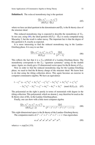
Now let us compute some dimensions of Ext groups between this twisted
cubic and its degree shifts by computing in the Landau–Ginzburg phase. This is
conveniently done using Macaulay 2.
i1 : kk = ZZ/31469
i2 : B = kk[x_0..x_4]
i3 : W = x_0ˆ5+x_1ˆ5+x_2ˆ5+x_3ˆ5+x_4ˆ5
i4 : A = B/(W)
i5 : M = coker matrix {{x_0+x_1,x_2+x_3,x_4}}
Now we use the internal Macaulay routine described in [28] to compute the
S -module ExtA .M; M /:4
i6 : ext = Ext(M,M)

o7 = cokernel {0, 0} | x_4 x_2+x_3 x_0+x_1 0 0 0 X_1x_3ˆ4
{-1, -1} | 0 0 0 x_4 x_2+x_3 x_0+x_1 0 ...
{-1, 3} | 0 0 0 0 0 0 0
{-2, 2} | 0 0 0 0 0 0 0

o7 : kk[X , x , x , x , x , x ]-module, quotient of (kk[X , x , x , x , x ,
4
x ])
1 0 1 2 3 4 1 0 1 2 3 4

We have suppressed part of the output. The first column of the output represents
the bi-degrees of the generators of this module. The first degree is the homological
degree discussed in the previous section, and the second degree is the original degree
associated to our graded ring B.
gr
Next we need to pass to the quotient category DSg .A/ by setting X1 D 1. This
collapses to a single grading as described above. The following code sets pr equal
to the map whose cokernel defines ExtA .M; M / above, and we define our rings S
and a singly graded B2.
i7 : pr = presentation ext
i8 : S = ring target pr
i9 : B2 = kk[x_0..x_4,Degrees=>{5:2}]

4
The Macaulay 2 variable X1 is our p. Note that Macaulay 2 views complexes in terms of
homology rather than cohomology and so X1 has R charge 2.


i10: toB = map(B2, S, {-1,x_0,x_1,x_2,x_3,x_4},
DegreeMap => ( i -> {-5*i#0+2*i#1}))

The last line above is the heart of our algorithm. It defines a ring map which sets
X1 D 1 and defines how we map degrees. It is now simple to compute the Ext’s
gr
in the quotient category DSg .A/ by constructing the tensor product:
i11 : extq = prune coker(toB ** pr)

o11 = cokernel {0} | x_4 x_2+x_3 x_0+x_1 0 0 0
x_3ˆ4 x_1ˆ4 0 0 |
{3} | 0 0 0 x_4 x_2+x_3 x_0+x_1 0
0 x_3ˆ4 x_1ˆ4 |
2
o11 : B2-module, quotient of B2

Finally we may compute the dimensions of spaces of morphisms in the D-brane
category by computing the dimensions of the above module at specific degrees.
This, of course, is the Hilbert function:
i12 : apply(20, i -> hilbertFunction(i, extq))

o12 = {1, 0, 2, 1, 3, 2, 4, 3, 3, 4, 2, 3, 1, 2, 0, 1, 0, 0, 0,
0}

o12 : List

The above list represents the dimensions of HomDgr .A/ .M; M hi i// for
Sg

Extk .M; M.r// D HomDgr .A/ .M; M h5k C 2ri/: (61)
Sg

Note that Serre duality implies HomDgr .A/ .M; M hi i// Š HomDgr .A/ .M; M
Sg Sg
h15 i i// which is consistent with the above output. For open strings beginning
and ending on the same untwisted 2-brane M , we immediately see

Ext0 .M; M / D C; Ext1 .M; M / D C2
Ext2 .M; M / D C2 ; Ext3 .M; M / D C: (62)

This shows that our twisted cubic curve has normal bundle Ø. 3/ ˚ Ø.1/.
We could also compute open string Hilbert spaces between M and twists of M .
For example, Ext1 .M; M.1// D C3 .

3.4 Hochschild Cohomology

The above computation in Macaulay also reveals the closed to open string map
Á .a/ from (5) in the case that a is the D-brane given by the line on the quintic

46 P.S. Aspinwall

in question. The closed string Hilbert space of Landau–Ginzburg theories has long
been understood [36]. For the quintic it is given by the quotient ring
CŒz0 ; z1 ; z2 ; z3 ; z4
Hc D D E : (63)
@f @f
@z0 ; : : : ; @z4

This was rederived in terms of Hochschild cohomology in [37, 38]. In our case
of the quintic, we are looking at a Z5 -orbifold of the Landau–Ginzburg theory. This
means that we should restrict attention to the subring of Hc invariant under Z5 . In
addition, when orbifolding, one needs to worry about additional contributions to the
Hilbert space coming from “twisted sectors.” This does not occur in the B-model
for the quintic.
The Hilbert space of closed strings in the quintic is therefore generated by
monomials in CŒz0 ; z1 ; z2 ; z3 ; z4 of degree 5d , for some integer d , where each
variable appears with degree Ä 3. As above, with the collapsing to a single degree,
this monomial corresponds to an element of Hochschild cohomology of degree 2d .
The closed to open string map Á .a/ therefore maps a Z5 -invariant polynomial
into a pair of matrices representing an endomorphism of the matrix factorization
corresponding to a. These endomorphisms must commute with all other matrices
representing elements of the open string Hilbert space according to (6).
But output o11 above tells us exactly the structure of Hom.a; aŒi / for any i .
The two rows tell us we have two generators. The ﬁrst one is obviously the identity
element in Hom.a; a/, and thus we denote it by 1.
If is a degree 5d monomial then Á .a/ is an element of HomDgr .A/ .M; M
Sg
h10d i//. If d D 0, we have the trivial case corresponding to the identity. If d D 1,
2 3 3 2
we have two elements x1 x3 1 and x1 x3 1. Clearly then

Á1 .a/ D 1
Áx 2 x 3 .a/ D x1 x3 1
2 3
1 3

Áx 3 x 2 .a/ D x1 x3 1:
3 2
(64)
1 3

For d > 1 the map is zero by degree considerations. The content of o11 thus fully
determines Á .a/. Methods of commutative algebra can thus be utilized to compute
the closed to open string map for the full untwisted sector for any model with a
Landau–Ginzburg orbifold phase.

4 Monodromy

The B-model data is dependent on the complex structure of X . Mirror to this
statement is the fact that the A-model data depends on a complexiﬁed K¨ hler
a
form B C iJ 2 H 2 .Y; C/. This statement suggests an interesting question about


monodromy. Suppose we consider a Lagrangian 3-cycle on Y . This defines a class
in H3 .Y; Z/. Now go around a loop in the moduli space of complex structures of Y .
This can have a nontrivial monodromy action on H3 .Y; Z/, and thus it must act on
the set of A-brane objects. We can think of H3 .Y; Z/ as the Grothendieck group for
the A-brane category. The corresponding Grothendieck group K.X / for B-branes
on a Calabi–Yau threefold5 is

K.X / D H 0 .X; Z/ ˚ H 2 .X; Z/ ˚ H 4 .X; Z/ ˚ H 6 .X; Z/: (65)

For mirror symmetry to work, there must be some action of monodromy in the
moduli space of complexified K¨ hler forms on the derived category and thus K.X /.
a
Part of this monodromy can be explained nicely in terms of the B-field. We
state this very briefly here and refer to [8] for a more complete description. The
B-field describes a 2-form flat gerbe connection on X for worldsheets with no
boundary. When boundaries are added, the gerbe connection restricts to a line
bundle connection on the boundary in some sense. This is exactly part of the bundle
data on D-branes. This intimate relationship between the B-field and the D-brane
bundle implies that a transformation B ! B C e, for some e 2 H 2 .X; Z/, must be
equivalent to a change in the bundle curvature F ! F C e.
Thus, monodromy associated to B C iJ ! .B C e/ C iJ maps any sheaf F to
the twisted sheaf F .De / where De is the divisor class dual to e. Such a twist by De
is an obvious automorphism of the derived category of X .
This monodromy preserves the decomposition (65). What about the other
monodromies? One may add further data, called a “stability condition,” to the
topological field theory. This is easier to explain in terms of the A-model. An
object in the Fukaya category is a Lagrangian 3-manifold in Y (with a line bundle
with a flat connection over it). This object is “stable” if it can be represented by a
special Lagrangian (see, e.g., [39]). As one moves in the moduli space of complex
structures, some objects in the Fukaya category will become unstable, and some
previously unstable objects may become stable. The monodromy action on the
Fukaya category will map the original stable set of objects to the new stable set
upon going around a loop in the moduli space. Accordingly, there must be some
similar story for the derived category where stability depends on the complexified
K¨ hler form [6, 40–42].
a
The monodromy B ! B C e can be viewed as monodromy around the
large radius limit. Consider the toric Calabi–Yau Z† with its r-fold multigraded
homogeneous coordinate ring S . Let .ei / denote a shift by one in the i th grading.
Now consider:
Definition 7. m† .ei / is the automorphism of the derived category Db .Z† / induced
by the action S.q/ ! S.q C ei /.

5
Let us assume the Calabi–Yau threefold is simply connected and the cohomology is torsion-free.

48 P.S. Aspinwall

That it is an automorphism follows from proposition 1, since it is obviously an
automorphism of Db .gr S /, and it is an automorphism of T† by the definition
of T† . In the Calabi–Yau phase it is easy to show that this monodromy indeed
corresponds to B ! B C e. It is argued from a physics point of view in [19]
that this is the correct automorphism to associate to any phase.

4.1 K-Theory

We will restrict analysis of monodromy to the K-theory associated to D-branes. Let
the K-theory class of S.q/ be represented by
q q r
K.S.q// D s1 1 s2 2 : : : sr :
q
(66)

Then the K-theory of Db .gr S / is obviously the additive group of Laurent polyno-
mials ZŒs1 ; s1 1 ; : : : ; sr ; sr 1 . The action of the automorphism S.q/ ! S.q C ei /
clearly corresponds to multiplication by si in this Laurent polynomial ring.
The K-theory of T† is invariant under such automorphisms and so must
correspond to an ideal. We can compute it as follows:
Proposition 8. Let B† D m_ m_ : : : and m_ D hx˛ ; xˇ ; x ; : : :i as in (18).
1 2 j
Define
fj D .1 t q˛ /.1 t qˇ /.1 tq / : : : ; (67)

where q˛ is the multidegree of x˛ , etc. Then

K.T† / D hf1 ; f2 ; : : :i: (68)

This result follows from Proposition 3. The fj ’s are the K-theory classes of m_
j
given by Koszul resolutions of m_ .
j
It follows that the K-theory for D-branes in a phase given by † is

ZŒs1 ; s1 1 ; : : : ; sr ; sr 1
K.Z† / D : (69)
K.T† /
We will call this the “monodromy ring” for phase †. In a smooth Calabi–Yau phase
it corresponds to the toric Chow ring.
Let us consider the K-theory and associated monodromy ring in the compact
case. Let M be an S=hWi-module. It typically has an infinite resolution in terms
of free S=hWi-modules. Thus we associate to any object a power series which
expresses the associated element of K-theory. It is convenient to include an extra
variable to express the R-grading.
Let P denote the ring of formal power series

ZŒŒs1 ; s1 1 ; s2 ; s2 1 ; : : : ; sr ; sr 1 ; ; 1
(70)


and define a map on free S=hWi-modules
v v
k.S=hWi.v/fmg/ D s11 s23 : : : sr r
v m
: (71)

By writing free S=hWi-module resolutions this extends to a map

k W Db .gr-S=hWi/ ! P: (72)

Ultimately the resolution of any object is periodic with period 2, and the product
of two consecutive maps, lifted to an S -module map, is of homological degree (and
hence R-degree since the two are identified) 2. It follows that for any object a, we
have
k.a/ D f .s1 ; s2 ; : : : ; sr ; /.1 C 2
C 4
C : : :/ C g.s1 ; s2 ; : : : ; sr ; /
f .s1 ; s2 ; : : : ; sr ; / (73)
D 2
C g.s1 ; s2 ; : : : ; sr ; /;
1
where f and g are finite polynomials. Clearly, it is the polynomial f that expresses
the K-theory information for DGrS.W/. Unfortunately this approach to K-theory is
not easy since the quotient by the K-theory of T† in (40) is awkward. Instead, we
will translate the monodromy statements about X† back to the noncompact case Z†
as we describe in an example in Sect. 4.3.

4.2 The GKZ System

The monodromy of integral 3-cycle D-branes of the A-model around loops in the
moduli space of complex structures is encoded in the Picard–Fuchs differential
equations. These in turn can be described torically in terms of the GKZ system [43–
45]. Let us simplify the discussion a little by assuming that X† is a hypersurface
in the toric variety. Also we will shift our indexing so that i D 0; : : : ; n 1;
j D 0; : : : ; d 1. The index i D 0 will correspond to the unique point in A properly
in the interior of the convex hull of A , and j D 0 corresponds to a row of 1’s in
the matrix A imposing the hyperplane condition. We write the partial differential
equations in terms of variables a0 ; : : : ; an 1 . Define the operators

X
n 1
@
Zj D ˛j i ai ˇj
i D0
@ai
(74)
YÂ @ Ãuj YÂ @ Ã uj
u D ;
u >0
@aj u <0
@aj
j j

where ˛j i are the entries in the matrix A and u is any vector with coordinates
.u0 ; u1 ; : : : ; un 1 / in the row space of the matrix ˆ. We also have

50 P.S. Aspinwall

(
. 1; 0; 0; : : :/ if i D 0
ˇi D (75)
0 otherwise.

A period, $, is then a solution of

Zj $ D u$ D0 (76)

for all j and u. The equations Zj $ D 0 can be used to replace the n variables
ai with r variables i . This is nothing other than going from the homogeneous
coordinate ring CŒa1 ; : : : ; an to a set of affine coordinates . 1 ; : : : ; r / on the toric
variety associated to the secondary fan. A choice of cone † in the secondary fan
corresponds to a phase and a choice of coordinates . 1 ; : : : ; r / [46].
The remaining differential equations u $ D 0 written in these affine coordi-
nates exhibit monodromy around the origin. This, according to mirror symmetry, is
exactly the same as the monodromy m† of Definition 7.
That this story works in the large radius Calabi–Yau phase has been understood
for some time. See, for example, [47]. An important point, which complicates the
analysis, is that the GKZ system does not give the full information on monodromy.
We will see that we need a systematic way of discarding “extra” solutions. The K-
theory picture of the monodromy ring above gives an interesting way of doing this,
which we now explore.

4.3 A Calabi–Yau and Landau–Ginzburg Example

Rather than exploring the full generalities of monodromy, it is easier to demon-
strate the general idea with an example. The quintic threefold and its associated
Landau–Ginzburg phase have been studied extensively, and the monodromy is well
understood (see, e.g., [8]). Here we discuss a slightly more complicated example
where the concept of the monodromy ring is more powerful.
Let the matrices A and ˆ be given by (written as AT jˆ):

Q1 Q2 Q3
p D x0 0 0 0 0 1 5 0 0 0
x1 1 0 0 0 1 1 1 0 0
x2 0 1 0 0 1 1 0 0 1
x3 0 0 1 0 1 1 0 0 1
(77)
x4 0 0 0 1 1 1 0 0 1
x5 5 3 3 31 0 0 1 2
x6 3 2 2 21 0 1 2 0
x7 1 1 1 11 1 2 1 0
x8 2 1 1 11 0 0 0 5


We have labeled each row by the associated homogeneous coordinate. A particular
simplicial decomposition of the corresponding pointset yields the canonical line
bundle of the weighted projective space P4 f5;3;3;3;1g .
The point in A corresponding to x8 is in the interior of a codimension one face of
the convex hull. This means that it should be completely irrelevant for our purposes,
and we will ignore it [46, 48]. As such we also ignore the last column of ˆ. The
first three columns are associated to charges giving the multigrading .Q1 ; Q2 ; Q3 /.
In this example we have r D 3, and thus the dimension of the moduli space of
complexified K¨ hler forms is 3.
a
To obtain a smooth hypersurface we may set
W D p.x1 x6 x7 C x2 C x3 C x4 C x5 x6 x7 /:
3 2 5 5 5 15 10 5
(78)
There are 12 possible triangulations of A (always ignoring x8 ), but we will
concentrate on only two of them. One of the triangulations corresponds to the
Calabi–Yau phase. The corresponding Stanley–Reisner ideal is
ICY D hx1 x5 ; x1 x6 ; x5 x7 ; x2 x3 x4 x6 ; x2 x3 x4 x7 i: (79)
The corresponding ideal we quotient by in (69) is

K.TCY / D h.1 s1 s2 /.1 s3 /; .1 s1 s2 /.1 s2 s3 2 /; .1 s3 /.1 s1 s2 2 s3 /;
.1 s1 /3 .1 s2 s3 2 /; .1 s1 /3 .1 s1 s2 2 s3 /i: (80)

The other is the Landau–Ginzburg phase with

ILG D hp; x6 ; x7 i
(81)
K.TLG / D h1 s1 5 ; 1 s2 s3 2 ; 1 s1 s2 2 s3 i:

In both of these phases we may choose a tilting collection consisting of 15
objects given by the union of fS. n; 0; 0/; S. n; 0; 1/; S. n; 1; 0/g for n D
0; : : : ; 4. This implies that the collection of monomials given by the union of
fs1 n ; s1 n s3 1 ; s1 n s2 1 g for n D 0; : : : ; 4 spans K.Z† / as a vector space. Let us
denote this collection of monomials T .
First consider the noncompact geometries Z† . Given any object in Db .Z† / we
can therefore find its class in K-theory by:
1. Find a free resolution of the object and thus express its K-theory class as a
Laurent polynomial in ZŒs1 ; s1 1 ; s2 ; s2 1 ; s3 ; s3 1 .
2. Reduce this polynomial mod K.T† / so that all its terms lie in T .

52 P.S. Aspinwall

This would be most easily done if there were some monomial ordering so that this
second step was reduction to the normal form. Sadly, there is no monomial ordering
that can do this.6
Moving to the compact examples X† we have a subtlety in that we do not know
precisely how to construct K.T† /. To evade this issue we work in the monodromy
ring of Z† . Let
i W XCY ! ZCY (82)

be the inclusion map for a Calabi–Yau phase. The key observation is that the
monodromy action given in Deﬁnition 7 is the same on X† as on Z† . Thus, if
we begin in the image of i , then we should expect to remain in the image of i .

4.4 Monodromy of the Structure Sheaf

We begin in the Calabi–Yau phase, where K.TCY / is given by (80). Consider the
structure sheaf ØX (i.e., i ØX ). This has a free resolution

f
0 G S. 5; 0; 0/
Q GS
Q G ØX G 0: (83)

This implies that ØX has a K-theory class 1 s1 5 as an object of the K-theory
of ZCY .
The quotient ring QŒs1 ; s1 1 ; : : :=K.TCY / is a vector space of dimension 15,
corresponding to the fact that the rank of the K-theory for Z† is 15. But
h1;1 .XCY / D 3, and so the rank of the K-theory is only 8. Consider the ideal in
QŒs1 ; s1 1 ; : : :=K.TCY / generated by 1 s1 5 . This is exactly the orbit of the structure
sheaf ØX under the action of the monodromy. Since monodromy is tensoring by
ØX .D/ for various divisors D, this will span the Chow ring of XCY . In this example,
over the rationals, the Chow ring gives the full even-dimensional cohomology and
thus the full K-theory.
We need the ideal generated by the image of the structure sheaf in the mon-
odromy ring of Z† . There is an exact sequence [49]

G R a
G R G R G 0;
0 (84)
.I W a/ I I C .a/

describing the image of a in R=I . This motivates the deﬁnition:

6
This is proven by showing that it is incompatible with any weight order.


Definition 8. The reduced monodromy ring is the quotient

QŒs1 ; s1 1 ; : : : ; sr ; sr 1
(85)
.K.T† / W OX /

where we have an ideal quotient in the denominator and OX is the K-theory class of
the structure sheaf.
This reduced monodromy ring is expected to describe the monodromy of X† .
In our case, using (80), the ideal quotient .K.T† / W OX / is easily computed using
Macaulay 2, but the result is rather messy. The important fact is that the degree of
this quotient is 8, exactly as expected.
It is more interesting to find the reduced monodromy ring in the Landau–
Ginzburg phase. It is easy to see that

QŒs1 ; s1 1 ; s2 ; s2 1 ; s3 ; s3 1 QŒs
Š 15 : (86)
K.TLG / hs 1i

This reflects the fact that it is a Z15 -orbifold of a Landau–Ginzburg theory. The
monodromy corresponds to the Z15 “quantum symmetry” acting on the moduli
space. Again, we clearly get a 15-dimensional vector space for the K-theory of ZLG .
Now in order to find the reduced monodromy ring for the Landau–Ginzburg
phase, we need to find the K-theory charge of the structure sheaf. We know how
to do that using the tilting collection above. This again becomes an exercise in
computer commutative algebra. We have an equivalence

1 s1 5 Š s1 4 s2 1 C 3s1 3 s2 1 s1 3 s3 1 3s1 2 s2 1 C 3s1 2 s3 1 C s1 1 s2 1
3s1 1 s3 1 3s1 4 C s3 1 C 4s1 3 4s1 2 C 3s1 1 .mod K.TCY //: (87)

The polynomial on the right is purely in terms of monomials with degree in the
tilting collection. This polynomial, which we denote , may therefore be used as the
K-theory class of ØX in the Landau–Ginzburg phase.
Finally, one can show with a little more computer algebra

QŒs1 ; s1 1 ; s2 ; s2 1 ; s3 ; s3 1 QŒs
Š 8 : (88)
.K.TLG / W / hs s7 C s5 s4 C s3 s C 1i

This eight-dimensional space is the K-theory of the Landau–Ginzburg theory.
The companion matrix of s 8 s 7 C s 5 s 4 C s 3 s C 1 has eigenvalues

˛; ˛ 2 ; ˛ 4 ; ˛ 7 ; ˛ 8 ; ˛ 11 ; ˛ 13 ; ˛ 14 ; (89)

where ˛ D exp.2 i=15/.

54 P.S. Aspinwall

The GKZ system has 15 linearly independent solutions. The above monodromy
around the Landau–Ginzburg point in the moduli space tells us which of the 8
solutions are pertinent for XLG . The older method for determining this would have
been to use intersection theory to establish the correct 8 solutions at large radius
limit and then analytically continue these solutions to the Landau–Ginzburg phase.
This method using the monodromy ring is much less arduous.

Acknowledgements I thank R. Plesser for many useful discussions. This work was partially sup-
ported by NSF grant DMS–0905923. Any opinions, findings, and conclusions or recommendations
expressed in this material are those of the author and do not necessarily reflect the views of the
National Science Foundation.

References

1. Grayson, D.R., Stillman, M.E.: Macaulay 2, a software system for research in algebraic
geometry. Available at http://www.math.uiuc.edu/Macaulay2/
´
2. Atiyah, M.: Topological quantum field theories. Inst. Hautes Etudes Sci. Publ. Math. 68,
175–186 (1989)
3. Lurie, J.: On the classification of topological field theories. In: Current Developments in
Mathematics, 2008, pp. 129–280. International Press, Somerville (2009). arXiv:0905.0465.
4. Douglas, M.R., Gross, M. (eds.): Dirichlet branes and mirror symmetry. Clay Mathematical
Monographs, vol. 4. American Mathematical Society, New York, Clay Mathematics Institute,
Cambridge (2009)
5. Witten, E.: Mirror manifolds and topological field theory. In: Yau, S.-T. (ed.) Essays on Mirror
Manifolds. International Press, Somerville (1992). hep-th/9112056
6. Douglas, M.R.: D-Branes, categories and N =1 supersymmetry. J. Math. Phys. 42, 2818–2843
(2001). hep-th/0011017
7. Aspinwall, P.S., Lawrence, A.E.: Derived categories and zero-brane stability. J. High Energy
Phys. 08, 004 (2001). hep-th/0104147
8. Aspinwall, P.S.: D-Branes on Calabi–Yau manifolds. In: Maldacena, J.M. (ed.) Progress in
String Theory. TASI 2003 Lecture Notes, pp. 1–152. World Scientific, Singapore (2005). hep-
th/0403166
9. Fukaya, K., Oh, Y.-G., Ohta, H., Ono, K.: Lagrangian Intersection Floer Theory—Anomaly
and Obstruction. (2000). http://www.math.kyoto-u.ac.jp/ fukaya/fukaya.html
10. Dijkgraaf, R., Verlinde, H.L., Verlinde, E.P.: Notes on topological string theory and 2-D
quantum gravity. In Green, M., et al. (eds.) String Theory and Quantum Gravity: Proceedings.
World Scientific, Singapore (1991). Proceedings of Trieste Spring School: String Theory and
Quantum Gravity, Trieste, Italy, Apr 23–1 May (1990)
11. Costello, K.: Topological conformal field theories and Calabi–Yau categories. Adv. Math. 210,
165–214 (2007). arXiv:math/0412149
12. To¨ n, B.: The homotopy theory of dg-categories and derived Morita theory. Invent. Math. 167,
e
615–667 (2007)
13. Oda, T., Park, H.S.: Linear Gale transforms and Gelfand–Kapranov–Zelevinskij decomposi-
tions. Tˆ hoku Math. J. 43, 375–399 (1991)
o
14. Cox, D.A.: The homogeneous coordinate ring of a toric variety. J. Algebraic Geom. 4, 17–50
(1995). alg-geom/9210008
15. Cox, D.A., Little, J.B., Schenck, H.K.: Toric varities. Graduate Studies in Mathematics,
vol. 124. American Mathematical Society, Providence (2010)


16. Hartshorne, R.: Algebraic geometry. Graduate Texts in Mathematics, vol. 52. Springer, New
York (1977)
17. Bondal, A., Orlov, D.: Semiorthogonal decomposition for algebraic varieties. alg-
geom/9506012
18. Witten, E.: Phases of N D 2 theories in two dimensions. Nucl. Phys. B403, 159–222 (1993).
hep-th/9301042
19. Herbst, M., Hori, K., Page, D.: Phases of N D 2 theories in 1 C 1 dimensions with boundary.
arXiv:0803.2045
20. Pantev, T., Sharpe, E.: String compactiﬁcations on Calabi–Yau stacks. Nucl. Phys. B733,
233–296 (2006). hep-th/0502044
21. Segal, E.: Equivalence between GIT quotients of Landau–Ginzburg B-models. Comm. Math.
Phys. 304, 411–432 (2011)
22. Miller, E., Sturmfels, B.: Combinatorial Commutative Algebra. Springer, New York (2005)
23. Aspinwall, P.S.: Topological D-branes and commutative algebra. Commun. Num. Theory.
Phys. 3, 445–474 (2009). hep-th/0703279
¸ˇ
24. Eisenbud, D., Mustata, M., Stillman, M.: Cohomology on toric varieties and local cohomology
with monomial supports. J. Symbolic Comput. 29, 583–600 (2000). arXiv:math/0001159
25. Van den Bergh, M.: Non-commutative crepant resolutions. In: The Legacy of Niels
Henrik Abel: The Abel Bicentennial, Oslo 2002, pp. 749–770. Springer, Berlin (2004).
arXiv:math/0211064
26. Aspinwall, P.S.: D-Branes on toric Calabi–Yau varieties. arXiv:0806.2612
27. Orlov, D.: Derived categories of coherent sheaves and triangulated categories of singularities.
In: Algebra, Arithmetic, and Geometry: in Honor of Yu.I. Manin. Vol. II. Progress in
Mathematics, vol. 270. pp. 503–531. Birkh¨ user, Boston (2009). math.AG/ 0506347
a
28. Avramov, L.L., Grayson, D.R.: Resolutions and cohomology over complete intersections. In:
Eisenbud, D., et al. (eds.) Computations in Algebraic Geometry with Macaulay 2, Algorithms
and Computations in Mathematics, vol. 8, pp. 131–178. Springer, New York (2001)
29. Gulliksen, T.H.: A change of ring theorem with applications to Poincare series and intersection
multiplicity. Math. Scand. 34, 167–183 (1974)
30. Eisenbud, D.: Homological algebra on a complete intersection, with an application to group
representations. Trans. Amer. Math. Soc. 260, 35–64 (1980)
31. Ballard, M., Favero, D., Katzarkov, L.: Variation of geometric invariant theory quotients and
derived categories. arXiv:1203.6643
32. Kapustin, A., Li, Y.: D-branes in Landau–Ginzburg models and algebraic geometry. J. High
Energy Phys. 12 005 (2003). hep-th/0210296
33. Hori, K., Walcher, J.: D-branes from matrix factorizations. Compt. Rendus Phys. 5, 1061–1070
(2004). hep-th/0409204
34. Ashok, S.K., Dell’Aquila, E., Diaconescu, D.-E., Florea, B.: Obstructed D-branes in Landau–
Ginzburg orbifolds. Adv. Theor. Math. Phys. 8, 427–472 (2004). hep-th/0404167
35. Aspinwall, P.S.: The Landau–Ginzburg to Calabi–Yau dictionary for D-branes, J. Math. Phys.
48, 082304 (2007). arXiv:hep-th/0610209
36. Vafa, C., Warner, N.: Catastrophes and the classiﬁcation of conformal theories. Phys. Lett.
218B, 51–58 (1989)
37. Kapustin, A., Rozansky, L.: On the relation between open and closed topological strings.
Commun. Math. Phys. 252, 393–414 (2004). arXiv:hep-th/0405232
38. Dyckerhoff, T.: Compact generators in categories of matrix factorizations. Duke Math. J. 159,
223–274 (2011). arXiv:0904.4713
39. Joyce, D.: Lectures on Calabi–Yau and special Lagrangian geometry. In: Global Theory of
Minimal Surfaces. Clay Mathematical Proceedings, vol. 2. American Mathematical Society,
Providence (2005). math.DG/0108088
40. Douglas, M.R., Fiol, B., R¨ melsberger, C.: Stability and BPS branes. J. High Energy Phys.
o
0509, 006 (2005). hep-th/0002037
41. Aspinwall, P.S., Douglas, M.R.: D-brane stability and monodromy. J. High Energy Phys. 05,
031 (2002), hep-th/0110071

56 P.S. Aspinwall

42. Bridgeland, T.: Stability conditions on triangulated categories. Ann. Math. (2) 166, 317–345
(2007). math.AG/0212237
43. Gel’fand, I.M., Zelevinski˘ A.V., Kapranov, M.M.: Hypergeometric functions and toral (toric)
ı
manifolds. Func. Anal. Appl. 23, 94–106 (1989). (from Russian in Funk. Anal. Pril. 23)
44. Gelfand, I.M., Kapranov, M.M., Zelevinski, A.V.: Discriminants, Resultants and Multidimen-
sional Determinants. Birkh¨ user, Basel (1994)
a
45. Batyrev, V.V.: Variations of the mixed hodge structure of afﬁne hypersurfaces in algebraic tori.
Duke Math. J. 69, 349–409 (1993)
46. Aspinwall, P.S., Greene, B.R., Morrison, D.R.: The monomial-divisor mirror map. Internat.
Math. Res. Notices 319–33 (1993). alg-geom/9309007
47. Hosono, S., Lian, B.H., Yau, S.-T.: GKZ-generalized hypergeometric systems in mirror
symmetry of Calabi-Yau hypersurfaces. Comm. Math. Phys. 182, 535–577 (1996). alg-geom/
9511001
48. Batyrev, V.V.: Dual polyhedra and mirror symmetry for Calabi–Yau hypersurfaces in toric
varieties. J. Alg. Geom. 3, 493–535 (1994)
49. Eisenbud, D.: Commutative algebra with a view towards algebraic geometry. Graduate Texts
in Mathematics, vol. 150. Springer, New York (2004)

Commutative algebra

Recommended

Recommended

More Related Content

What's hot

What's hot (19)

Similar to Commutative algebra

Similar to Commutative algebra (20)

More from Springer

More from Springer (20)

Commutative algebra