This document provides a summary of a master's thesis in mathematics. The thesis studies generalisations of the fact that every Riesz homomorphism between spaces of continuous functions on compact Hausdorff spaces can be written as a composition multiplication operator. Specifically, the thesis examines Riesz homomorphisms between spaces of extended continuous functions on extremally disconnected spaces, known as Maeda-Ogasawara spaces. It proves that every Riesz homomorphism on such a space has a generalized composition multiplication form involving a continuous map between the underlying spaces. The thesis also applies these results to spaces of measurable functions and explores Riesz homomorphisms between spaces of continuous functions with values in a Banach lattice.


![1
1 Introduction
This thesis finds its conception as a crossbreed of two others, namely [21] of H. van Imhoff and
[20] of B. van Engelen. After asking Dr. Van Gaans and Prof. Van Rooij to be my supervisors,
they each contributed one of them as inspiration for my choice of subject. In the first of the
two, we find a study on ways to generalise a characterisation of Riesz homomorphisms on spaces
of continuous functions to specific subspaces. In the second one, lattice isomorphisms instead
of Riesz homomorphisms are treated, among others on spaces of extended continuous functions.
The classic Maeda-Ogasawara Theorem plays an important role there.
In this thesis, the two subjects are combined. After a section on preliminary Riesz space theory,
Section 3 concerns the same characterisation as studied in [21], but now for Riesz homomor-
phisms on spaces of extended continuous functions.
The classical theorem on which [21] builds, can for example be found as Theorem 2.34 in [3].
Theorem. Let X and Y be compact Hausdorff spaces and let T : C(X) → C(Y ) be a positive
operator. Then T is a Riesz homomorphism if and only if there exist a map π : Y → X and a
function η ∈ C(Y )+ such that for all f ∈ C(X): Tf = η(f ◦ π). In this case, η = T1X and π
is uniquely determined and continuous on {η > 0}.
C(X) C(Y ) T1X =: ηT
π
Operators of the form f → η(f ◦ π) are called composition multiplication operators.
The extended continuous functions on an extremally disconnected compact Hausdorff space X,
of which a precise definition is given in Section 2, form a Riesz space, which is denoted by
C∞(X). The Maeda-Ogasawara Theorem implies that every Archimedean Riesz space E can be
embedded as an order dense Riesz subspace in some C∞(X), called its Maeda-Ogasawara space.
If we also embed the image of E in a C∞(Y ), this yields a pointwise description that allows
us to study whether a Riesz homomorphism on E is in any sense of composition multiplication
form.
Outline
In Section 2, we will quickly introduce the necessary terminology and notation, referring to
standard literature on Riesz spaces for the details. After this, Section 3 contains the principal
part of the thesis, where we will expand the theory of generalised multiplication operators on
Maeda-Ogasawara spaces.
Both for the sake of clarity and to refrain from repetition, most subsections start with a
sketch of the situation at hand, displayed in a frame.
A typical example of an extremally disconnected compact Hausdorff space is βN, the Stone-ˇCech
compactification of the natural numbers. Therefore, we begin Section 3 by proving some results
on Riesz homomorphisms on C∞(βN), motivating our line of thought.
We proceed by studying the general setting of a Riesz subspace E ⊂ C∞(X), where in most
cases we may safely assume E is a Riesz ideal in C∞(X).
In Section 3.2, we find a generalised composition multiplication form satisfied by all Riesz ho-
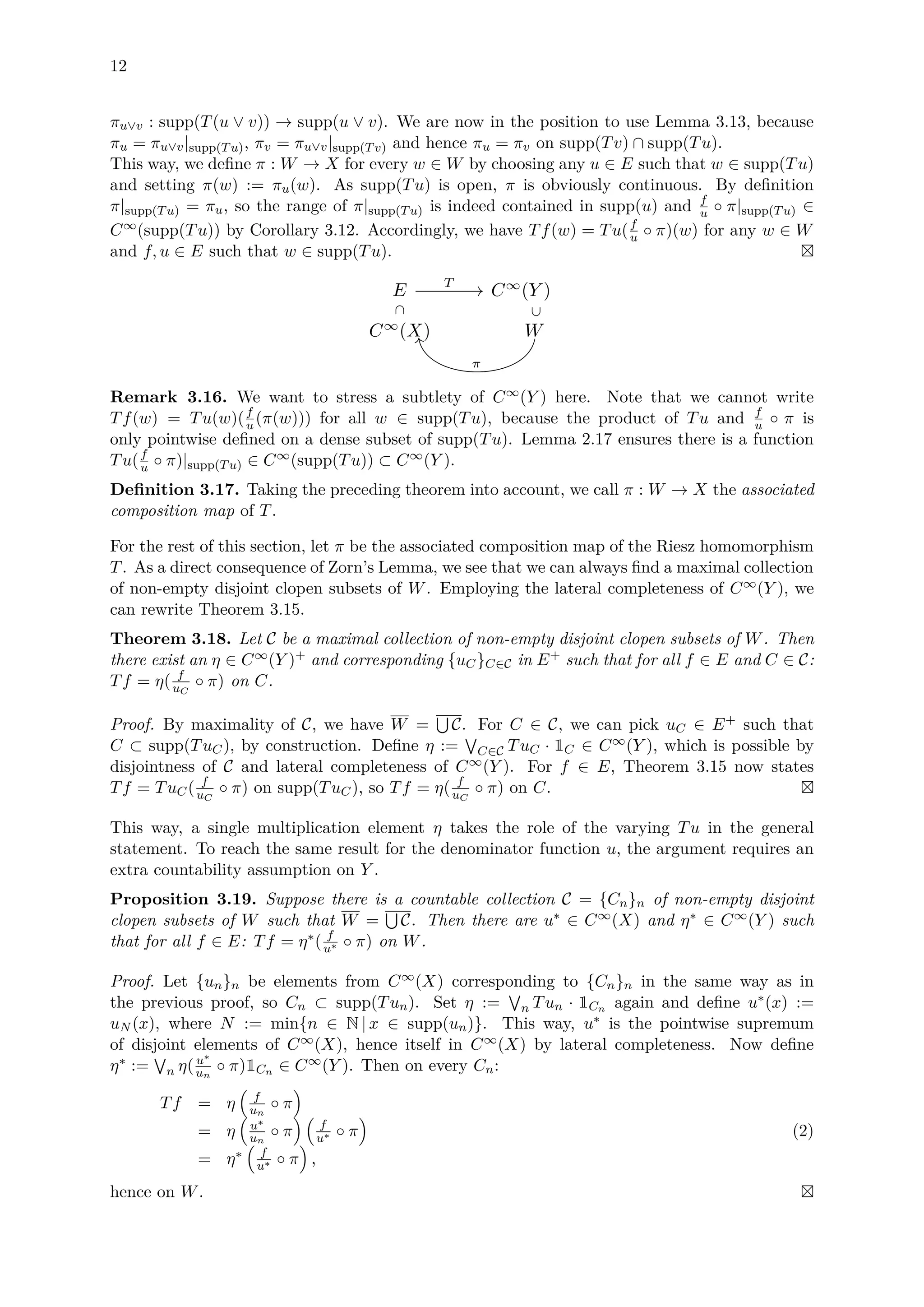
momorphisms on E, which is stated in Theorem 3.15. We call the continuous map Y → X
resulting from this the associated composition map of the Riesz homomorphism. The theorem](https://image.slidesharecdn.com/7a110103-c215-45ff-8349-ca9740682412-160901090557/75/Masterscriptie-T-Dings-4029100-7-2048.jpg)
![2
can be tweaked in all kinds of ways, already with an eye on the situation where C∞(X) is the
Maeda-Ogasawara space of E.
In Section 3.3, we explore ways to limit the sometimes counter-intuitive behaviour of C∞(X)
by imposing extra requirements on the way the Riesz homomorphism treats order limits.
We proceed by examining the properties of the associated composition map. Section 3.4 proves
the relationship between injectivity and surjectivity of the map and its Riesz homomorphism.
To conclude the reasoning, Section 3.5 summarises the results and connects them to the explicit
setting where C∞(X) is the Maeda-Ogasawara space of E.
Finally, we study an example of the theory. Spaces of measurable functions provide a natural
setting to apply the results, as the Maeda-Ogasawara space of the familiar Lp spaces is Riesz
isomorphic to the whole space of measurable functions on the same σ-finite measure space. This
also brings us back to the second part of [21], where the same matter is studied.
Wondering whether there are more ways to exploit the methods of this thesis, we take Section 4
to explore Riesz homomorphisms from C(X; E) to C(Z), where X, Z are realcompact Hausdorff
spaces and E is a Banach lattice. In this case, there indeed proves to be another kind of gener-
alised composition multiplication form, of which the main results are summarised in Theorem
4.15.
In the last part of this thesis, we comment on the content and possible directions for further
research in Section 5. Section 6 provides a Dutch summary in layman’s terms, in which we try
to bring across the subject in a way that is comprehensible for people without a mathematical
background.2
2
Whether this is successful is left for others to decide.](https://image.slidesharecdn.com/7a110103-c215-45ff-8349-ca9740682412-160901090557/75/Masterscriptie-T-Dings-4029100-8-2048.jpg)
![3
2 Preliminary Riesz space theory
Let us ensure we are all on the same page regarding the basic concepts and definitions. Every-
thing can be found in Chapter 1 of [11] unless otherwise stated, and we refer to this source for
details.3
Definition 2.1. A Riesz space is an ordered vector space with a lattice structure, meaning that
every non-empty finite subset of the space has an infimum and a supremum in the space.
Notation 2.2. Let E be a Riesz space and take f, g ∈ E. We write f ∨ g := sup{f, g},
f ∧ g := inf{f, g}, f+ := f ∨ 0, f− := (−f) ∨ 0, |f| := f ∨ (−f), and E+ := {f ∈ E | f ≥ 0}
(which we call the positive cone of E).
Remark 2.3. Although it seems natural to think of a Riesz space as a lattice with nodes,4 a
typical example is C(X), the space of continuous functions on a topological space X.5
Definition 2.4. An element e ∈ E+ is
(i) a strong unit if for every f ∈ E there exists an n ∈ N with |f| ≤ ne;
(ii) a weak unit if for every f ∈ E: |f| ∧ e = 0 implies that f = 0.
Every strong unit is obviously also a weak unit.
We list a few additional properties Riesz spaces may possess.
Definition 2.5. A Riesz space E is
(i) unitary if it contains a strong unit;
(ii) Archimedean if the set of f ∈ E+ for which {nf | n ∈ N} is bounded contains only 0;
(iii) (σ-)Dedekind complete if every (countable) non-empty subset which is bounded from above
has a supremum;
(iv) laterally complete if every non-empty disjoint subset of E+ has a supremum.
Definition 2.6. A linear subspace D of a Riesz space E is
(i) a Riesz subspace if f, g ∈ D implies that f ∨ g, f ∧ g ∈ D;
(ii) a Riesz ideal if f ∈ D, g ∈ E, |g| ≤ |f| together imply that g ∈ D;
(iii) majorising if for every f ∈ E+, there exists a g ∈ D+ such that f ≤ g;
(iv) order dense if for every non-zero f ∈ E+, there exists a g ∈ D+ such that 0 < g ≤ f.
We immediately see that every Riesz ideal is a Riesz subspace.
Natural objects to study in this context are maps that preserve the Riesz structure.
Definition 2.7. Let E, F be Riesz spaces. A map E → F is a Riesz homomorphism if it is both
linear and a lattice homomorphism. A bijective Riesz homomorphism is a Riesz isomorphism.
E and F are Riesz isomorphic if there exists a Riesz isomorphism E → F, in which case we
write E ∼= F.
We shall need one more notion that combines some of the concepts introduced above. We state
a classical theorem, which can be found in [11] as Theorem 32.5.
Theorem 2.8 (Nakano-Judin). Let E be an Archimedean Riesz space. Then there exists a
unique Dedekind complete Riesz space Eδ such that E is Riesz isomorphic to some majorising
order dense subspace of Eδ. Eδ is the Dedekind completion of E.
Under the embedding f → fδ of E into Eδ, for each h ∈ Eδ we have
sup{f ∈ E | fδ
≤ h} = h = inf{g ∈ E | gδ
≥ f}.
3
If possible, the reader may also want to consult [22] for a more accessible introduction.
4
such as R2
with the natural ordering (x1, x2) ≤ (y1, y2) if x1 ≤ y1 and x2 ≤ y2
5
The well-known Yosida Theorem, presented in Chapter 3 of [22], illustrates this.](https://image.slidesharecdn.com/7a110103-c215-45ff-8349-ca9740682412-160901090557/75/Masterscriptie-T-Dings-4029100-9-2048.jpg)
![4
Notation 2.9. We identify E with the embedding in its Dedekind completion and write E ⊂ Eδ.
As mentioned in the beginning, C(X) for a topological space X is the classical example of a
Riesz space. We cite two well-known results in the field, Theorems 2.33 en 2.34 from [3], that
motivate the rest of this thesis. Theorem 2.11 is a generalisation of the Banach-Stone Theorem.
Lemma 2.10. Let X = ∅ be compact Hausdorff and let φ : C(X) → R be a Riesz homomor-
phism. Then there is an x0 ∈ X such that φ(f) = φ(1)f(x0) for all f ∈ C(X), so φ is a multiple
of an evaluation.
Theorem 2.11. Let X and Y be compact Hausdorff spaces and let T : C(X) → C(Y ) be a
positive operator. Then T is a Riesz homomorphism if and only if there exist a map π : Y → X
and a function η ∈ C(Y )+ such that for all f ∈ C(X): Tf = η(f ◦ π). In this case, η = T1X
and π is uniquely determined and continuous on {η > 0}.
C(X) C(Y ) T1X =: ηT
π
Definition 2.12. An operator of the form f → η(f ◦ π) is called a composition multiplication
operator,6 abbreviated as cm-operator in the sequel.
In [21], we find extensions of Theorem 2.11 to both pre-Riesz spaces with Riesz* homomorphisms
and to spaces of measurable functions. We shall not go into this any deeper at this point, but
will come back to the latter in Section 3.6.
This thesis aims to extend and generalise Theorem 2.11 in two other ways. For the first of these,
we study the representation theorem of Maeda-Ogasawara. Before we introduce the result,
however, we have to define the notion of an extended continuous function on an extremally
disconnected compact Hausdorff space. We follow Chapter IV.15 of [5] and Chapter 7 of [11],
which the reader may consult for the proofs of the cited results and an elaboration on the topic.
Definition 2.13. Let X be a topological space. A subset A of X is
(i) clopen if it is both open and closed;
(ii) dense if A = X;
(iii) meagre if there exist closed subsets C1, C2, . . . ⊂ X such that C◦
n = ∅ and A ⊂ n Cn.
X is extremally disconnected if the closure of every open set is open (hence clopen).
It is clear that the complement of a meagre set is dense. An equivalent definition of extremal
disconnectedness is that every two disjoint open subsets of X have disjoint closures.
Definition 2.14. The extended real numbers consist of the set R := R∪{±∞} with the canonical
ordering and topology (such that tan : [−1
2π, 1
2π] → R is a homeomorphism).
Definition 2.15. The space of extended continuous functions on an extremally disconnected
compact Hausdorff space X consists of all continuous functions f : X → R such that f−1({±∞})
is meagre, and is denoted by C∞(X).
Remark 2.16. We could have defined C∞(X) for any topological space X, but the above
construction does in general not yield a Riesz space.
Lemma 2.17. Let B ⊂ X be dense, and suppose f : B → R is continuous. Then f has a unique
extension in C∞(X).
6
or weighted composition operator](https://image.slidesharecdn.com/7a110103-c215-45ff-8349-ca9740682412-160901090557/75/Masterscriptie-T-Dings-4029100-10-2048.jpg)
![5
For f, g ∈ C∞(X), the closed set A := {f = ±∞} ∪ {g = ±∞} is meagre. Hence X A is dense,
and we define f + g, fg : X A → R by (f + g)(x) := f(x) + g(x) and fg(x) = f(x)g(x). The
previous lemma leads to unambiguous extensions of f + g and fg in C∞(X).
Theorem 2.18. The space C∞(X) with these operations, supplemented by the natural ordering
and scalar multiplication, is a multiplicative, Dedekind complete, and laterally complete Riesz
space.
Remark 2.19. The constant function 1X is a strong unit in C(X), but a weak unit in C∞(X).
Definition 2.20. For future purposes, we also define the quotient f
g of f, g ∈ C∞(X) to be the
unique continuous extension of
x →
f(x)
g(x) on {g > 0} A
0 on {g > 0}
c
,
to the whole X, where A := {f = ±∞} ∪ {g = ±∞} ∪ {g = 0} is meagre in {g > 0}. We call
the set {g > 0} the support of g and write supp(g) for it.
Note that by extremal disconnectedness, the support of any function in C∞(X) is clopen. In
addition, we see that f
g g = f1supp(g) ≤ f for f ≥ 0.
We now come to the main point: the next theorem clarifies why these spaces are of interest.
Theorem 2.21 (Maeda-Ogasawara). Let E be an Archimedean Riesz space. Then there exists
a unique extremally disconnected compact Hausdorff space X such that E is Riesz isomorphic
to an order dense subspace of C∞(X). C∞(X) is called the Maeda-Ogasawara space of E. If
E contains a weak unit e, there is an embedding under which e is mapped to 1X.
Notation 2.22. We also identify E with the embedding in its Maeda-Ogasawara space C∞(X)
and write E ⊂ C∞(X).
To provide a connection between the Dedekind completion and the Maeda-Ogasawara space of
E, we adapt Theorem 1.40 from [2] and Corollary 32.8 from [11] to the present setting.
Lemma 2.23. Let D ⊂ E be an order dense Riesz subspace of an Archimedean Riesz space E.
If D is Dedekind complete in its own right, then D is a Riesz ideal of E.
Corollary 2.24. If E is an Archimedean Dedekind complete Riesz space, then the embedding
E ⊂ C∞(X) in its Maeda-Ogasawara space is a Riesz ideal.
Lemma 2.25. Let D ⊂ E be a Riesz subspace of an Archimedean Dedekind complete Riesz
space E, such that D is order dense in the Riesz ideal D ⊂ E generated by D. Then D = Dδ.
Corollary 2.26. Let E be an Archimedean Riesz space. Suppose Eδ is its Dedekind completion,
C∞(X) is its Maeda-Ogasawara space and E is the Riesz ideal generated by E in C∞(X). If
E ⊂ E is order dense, then E ∼= Eδ.
In particular, if E is an ideal, so E = E , then E is its Eδ and is hence Dedekind complete.
To finish this discussion, let us present the result of Theorem 1.50(a) from [2] as an example.
Example 2.27. If X is an extremally disconnected compact Hausdorff space, then C(X) ⊂
C∞(X) is the Riesz ideal generated by the Riesz subspace of step functions
D :=
N
n=1
λn1Un | λn ∈ R, Un ⊂ X clopen .
D ⊂ C(X) is order dense, so C(X) = Dδ and C(X) is Dedekind complete.](https://image.slidesharecdn.com/7a110103-c215-45ff-8349-ca9740682412-160901090557/75/Masterscriptie-T-Dings-4029100-11-2048.jpg)
![6
The extremally disconnected spaces mentioned in the preceding may be considered somewhat
counter-intuitive. Throughout this text, the Stone-ˇCech compactification of the natural numbers
is often raised as an example. We state the basics and refer to chapter 4 of [22] for more
information.
Theorem 2.28. Let X be a completely regular space and K a compact Hausdorff space. Then
there is a unique compact Hausdorff space, denoted by βX, with a continuous map β : X → βX
such that
(i) X is homeomorphic via β to a dense subset β(X) ⊂ βX;
(ii) every continuous map f : X → K lifts to a unique continuous map f : βX → K with
f = β ◦ f .
X K
βX
β
f
f
Definition 2.29. The space βX is called the Stone- ˇCech compactification of X,
Proposition 2.30. βN has the following properties:
(i) the space is extremally disconnected;
(ii) the singleton {β(n)} is clopen for every n ∈ N;
(iii) if x ∈ β(N), then f(x) ∈ R for every f ∈ C∞(βN);
(iv) if we define j ∈ C∞(βN) to be the unique continuous extension of β(n) → n ∈ R, then
j(x) = ∞ for every x ∈ βN β(N).
To conclude this section of preliminaries, we remark that the definitions and constructions
above mainly concern Section 3. The necessary background on measurable functions is men-
tioned briefly in Section 3.6, and in Section 4, a few additional notions are introduced when
appropriate.](https://image.slidesharecdn.com/7a110103-c215-45ff-8349-ca9740682412-160901090557/75/Masterscriptie-T-Dings-4029100-12-2048.jpg)
![8
Now let a ∈ βN β(N). We have a net (xι)ι in β(N) converging to a, so using continuity of Tf,
f, and π, we see that
(Tf)(a) = (Tf)(limι xι)
= limι(Tf)(xι)
= limι f(˜π(xι))
= limι f(π(xι))
= f(π(limι xι))
= f(π(a)).
We conclude that π : βN → βN is a continuous map such that Tf = f ◦ π, as desired.
We immediately recognise a difference between C(X) and C∞(X).
Remark 3.3. Not every continuous π : βN → βN yields a Riesz homomorphism C∞(βN) →
C∞(βN) via f → f ◦ π. Fix for example a ∈ βN β(N) and define π(x) := a for every x ∈ βN.
If f(a) = ∞, then f ◦ π /∈ C∞(X).
Furthermore, we can not hope for every Riesz homomorphism to be a cm-operator, considering
the situation where 1 /∈ E ⊂ C∞(βN).
Example 3.4. Define j ∈ C∞(βN) as in Proposition 2.30(iv) and pick a ∈ βNβ(N) arbitrarily.
Let E ⊂ C∞(βN) be given by E := {f ∈ C∞(βN) | (fj)(a) ∈ R} and T : E → C∞({0}) ∼= R by
Tf = Tf(0) := (fj)(a). Then 1
j ∈ E and T 1
j = 1, so T = 0.
Suppose Tf = η(f ◦ π) for some η ∈ R+, π : {0} → βN. Note that η must be real, because {0}
is clopen. For g ∈ C(βN), g
j ∈ E. Then g(a) = T g
j = η(g
j ◦ π). We have π(0) = a, for if not,
we can find an open U ⊂ βN with a ∈ U ∈ π(0). For g := 1U , this means that g(a) = 1, while
g
j (π(0)) = 0, which is a contradiction.
Hence Tf = ηf(a), but f(a) = 0 for all f ∈ E, implying Tf = 0. This is again a contradiction,
from which we conclude such η and π do not exist.
With these examples in mind, we proceed by studying the abstract setting of a Riesz subspace
E ⊂ C∞(X) and a Riesz homomorphism T : E → C∞(Y ), where both X and Y are extremally
disconnected compact Hausdorff spaces. We preferably work with Riesz ideals, so the next
result, Theorem 2.29 of [3], is of great use.
Theorem 3.5 (Lipecki-Luxemburg-Schep). Let E, F be Riesz spaces, F Dedekind complete,
and let A ⊂ E be a majorising Riesz subspace with a Riesz homomorphism T : A → F. Then
there exists a (not necessarily unique) Riesz homomorphism T : E → F extending T.
Corollary 3.6. Let E ⊂ C∞(X) be a Riesz subspace, E the ideal generated by E in C∞(X)
and T : E → C∞(Y ) a Riesz homomorphism. Then there is a Riesz homomorphism T : E →
C∞(Y ) extending T.
Proof. C∞(Y ) is Dedekind complete and E is majorised by E.
E
E C∞
(Y )
C∞
(X)
T
⊂
T
⊂
Hence we may assume E is an ideal, as long as we do not impose any further requirements on
T (see Section 3.3).
Remark 3.7. To see the existence of such an extension is generally false for non-majorising
subspaces, we refer to Remark 3.3: for the given continuous map π : βN → βN, f → f ◦ π is a
Riesz homomorphism from C(βN) → C(βN) that can not be extended to the whole C∞(βN).](https://image.slidesharecdn.com/7a110103-c215-45ff-8349-ca9740682412-160901090557/75/Masterscriptie-T-Dings-4029100-14-2048.jpg)


![13
To put this assumption into context, let us mention the following.
Definition 3.20. If every collection of non-empty disjoint open sets of a topological space is
at most countable, the space has the Suslin property.7 This is also called the countable chain
condition.
Informally speaking, one could say that a space with the Suslin property is sufficiently small to
contain only a countable number of disjoint non-negligible sets.
Remark 3.21. In an extremally disconnected space, open sets are disjoint if and only if their
closures are. We can therefore replace ‘open’ by ‘clopen’ when assuming an extremally discon-
nected space has the Suslin property.
If Y has the Suslin property, it naturally satisfies the assumptions of Proposition 3.19.
Example 3.22. Considering Suslin’s problem, it is not surprising that R has the Suslin property.
It is easy to see that βN does as well. The property is closely related to Section 3.6, in which the
application of the results of this section to spaces of measurable functions on σ-finite measure
spaces is studied.
Let us defer this analysis of the Suslin property for now and turn back to our general line of
thought. We can also answer a natural question about composition of Riesz homomorphisms
and their associated composition maps.
Proposition 3.23. Let F ⊃ T(E) be a Riesz ideal of C∞(Y ) and let Z be a extremally dis-
connected compact Hausdorff space. Suppose S : F → C∞(Z) is a Riesz homomorphism.
Set V := g∈F supp(Sg). Let σ : V → Y be the associated composition map of S and
τ : f∈E supp(STf) =: V → X the associated composition map of ST. Then τ and π ◦ σ
coincide on V .
Proof. Choose f, u ∈ E arbitrarily. Using Theorem 3.15, we see that σ(supp(STu)) ⊂ supp(Tu),
so on supp(STu):
STu f
u ◦ τ = STf
= STu Tf
Tu ◦ σ
= STu
Tu(f
u
◦π)
Tu ◦ σ
= STu f
u ◦ π ◦ σ , so
f
u ◦ τ = f
u ◦ π ◦ σ.
(3)
Suppose τ(z0) = π(σ(z0)) for some z0 ∈ V . Then there is some u ∈ E with z0 ∈ supp(STu),
so both τ(z0), π(σ(z0)) ∈ supp(u). Take a clopen U ⊂ supp(u) such that τ(z0) ∈ U ∈ π(σ(z0)).
Define f ∈ E by f(x) := 0 for x ∈ U and f := u outside. Then f
u (τ(z0)) = 0 = 1 = f
u (π(σ(z0)),
contradicting (3).
In the context of the Maeda-Ogasawara Theorem 2.21, to which we will turn later on in this
section, order dense subspaces of C∞(X), C∞(Y ) are of interest. We mention some implications.
Lemma 3.24. Let E ⊂ C∞(X) be an order dense Riesz subspace (so not necessarily an ideal).
Then N(E) is meagre.
7
The Suslin property is closely related to Suslin’s problem. Suppose R is a non-empty totally ordered set
without a least or greatest element, on which the order is dense and complete, and which has the Suslin property.
Must R be order isomorphic to R? It is proved in [17] that this hypothesis is independent of zfc.](https://image.slidesharecdn.com/7a110103-c215-45ff-8349-ca9740682412-160901090557/75/Masterscriptie-T-Dings-4029100-19-2048.jpg)


![16
Proof. By Lemma 3.34, we have f ◦ π|supp(Tf), g ◦ π|supp(Tg) ∈ C∞(Y ). Theorem 3.15 yields
g
f ◦ π|supp(Tf) ∈ C∞(supp(Tf)), so in particular on a dense subset D ⊂ supp(Tf) ∩ supp(Tg):
g
f ◦π = g◦π
f◦π =: h. Observe that h(y) can only be infinite when g(π(y)) = ∞ or f(π(y)) = 0. Both
sets are meagre, because g◦π|supp(Tg) ∈ C∞(Y ) and π(supp(Tf)) ⊂ supp(f). Hence h|supp(Tf) ∈
C∞(supp(Tf)) and h = g
f ◦π on supp(Tf). This leads to Tg = (Tf)h, so (Tg)(f◦π) = (Tf)(g◦π)
on supp(Tf) ∩ supp(Tg).
To pursue all of this (and even more, as we will see later on), we study a particular class of Riesz
homomorphisms.
Definition 3.36. An operator S : E → F is (σ-)order continuous if it preserves order limits. In
other words: if for every increasing net(/sequence) (xι)ι in E with supι xι = x ∈ E: supι Sxι =
Sx.8
We remark that any Riesz isomorphism is obviously order continuous. Let us first relate this to
Lemma 3.34.
Proposition 3.37. Suppose T is σ-order continuous. If f, g ∈ E with supp(f) ⊂ supp(g), then
supp(Tf) ⊂ supp(Tg).
Proof. Let f, g ∈ E with supp(f) ⊂ supp(g). Then f = n(f ∧ ng), so Tf = n(Tf ∧ nTg).
We conclude Tf = 0 outside supp(Tg), so supp(Tf) ⊂ supp(Tg).
Remark 3.38. Up until this point, we have assumed E to be an ideal, because a Riesz homo-
morphism E → C∞(Y ) can be extended to the ideal E generated by E in C∞(X) using the
Lipecki-Luxemburg-Schep Theorem 3.5. Note, however, that extra properties of the homomor-
phism, such as (σ-)order-continuity, may not be preserved.
We provide an example to illustrate that σ-order continuity is not always preserved.
Example 3.39. Let R ∼= E ⊂ C[0, 1] be the Riesz subspace of constant functions, so the ideal E
generated by E is equal to the whole C[0, 1]. The identity λ1 → λ clearly is an order-continuous
Riesz homomorphism from E to R. The evaluation φa : C[0, 1] → R for any a ∈ [0, 1] extends
the identity, but is not σ-order continuous: the sequence of triangular spikes tn ∈ C[0, 1] on
[a − 1
n , a + 1
n ] ∩ [0, 1] with tn(a) = 1 for all n converges to the zero function, while φa(tn) = 1 for
all n.
3.3.1 Order continuous operators
We proceed by studying order continuous Riesz homomorphisms, in which case the situation
turns out to be less complicated.
In this subsection, E ⊂ C∞(X) is Riesz subspace, not necessarily a Riesz ideal, and T :
E → C∞(Y ) is order continuous. That means the results of the previous sections do not
immediately apply, because we required E to be a Riesz ideal there. We do assume that
both E ⊂ C∞(X) and T(E) ⊂ C∞(Y ) are order dense. Being the natural outcome of the
application of the Maeda-Ogasawara Theorem, we argue this is not such a strong assumption.
Lemma 3.40. There exists an order continuous Riesz homomorphism Tδ : Eδ → C∞(Y )
extending T.
8
This is clearly equivalent to: for every decreasing net(/sequence) in E+
converging to zero, the sequence of
images also converges to zero.](https://image.slidesharecdn.com/7a110103-c215-45ff-8349-ca9740682412-160901090557/75/Masterscriptie-T-Dings-4029100-22-2048.jpg)
![17
Proof. Pick h ∈ Eδ and define A := {f ∈ E | f ≤ h} and B := {g ∈ E | g ≥ h}. We have
sup(A) = h = inf(B), or inf(B − A) = 0 (viz. Theorem 2.8). Applying T, order-continuity
yields 0 = T(inf(B − A)) = inf(T(B) − T(A)) = inf(T(B)) − sup(T(A)) and sup(T(A)) =
inf(T(B)) =: Tδh yields the desired operator.
It is easy to see that Tδ is a Riesz homomorphism. To see Tδ is order continuous, let (hι)ι be
an increasing net in Eδ, converging to h ∈ Eδ. Tδhι ≤ Tδh for all ι, so supι Tδhι ≤ Tδh. By
Dedekind completeness, supι Tδhι exists in C∞(Y ). Using order continuity of T, we then have
supι Tδhι = supι sup{Tf ∈ C∞(Y ) | f ≤ hι}
= sup{Tf ∈ C∞(Y ) | f ≤ supι hι}
= sup{Tf ∈ C∞(Y ) | f ≤ h}
= Tδh.
We conlude Tδ is an order continuous Riesz homomorphism.
Order continuity of T allows us to consider the Dedekind completion of E. Theorem 2.32 from
[3] covers that. For future reference, we also cite the supporting Lemma 23.15 from [1].
Lemma 3.41. Let D be an Archimedean Riesz space and A ⊂ D a Dedekind complete, order
dense Riesz subspace. Then every element of D+ is the supremum of a disjoint system of
elements of A+.
Theorem 3.42. Let T : A → D be an order continuous Riesz homomorphism from a Dedekind
complete Riesz space A to an Archimedean laterally complete Riesz space D. If A is an order
dense Riesz subspace of an Archimedean Riesz space B, then
˜T(x) := sup{T(y) | y ∈ A, 0 ≤ y ≤ x} (5)
defines an extension of T from B+ (and hence B) to D, which is an order continuous Riesz
homomorphism.
In the context of this thesis, the theorem proves the following.
Corollary 3.43. There exist η ∈ C∞(Y ) and a unique π : Y → X such that f ◦ π ∈ C∞(Y )
and Tf = η(f ◦ π). Furthermore, the map π is continuous.
Proof. We first form the Dedekind completion Eδ of E, with its associated order continuous
Tδ : Eδ → C∞(Y ) resulting from Lemma 3.40. E ⊂ Eδ ⊂ C∞(X) is order dense and Eδ is
Dedekind complete, so the previous theorem yields an extension ˜T : C∞(X) → C∞(Y ) of Tδ.
Define η := ˜T1X and Y0 := supp(η). Applying Corollary 3.9, we have a unique π : Y0 → X,
which is continuous, such that f ◦ π ∈ C∞(Y0) and ˜Tf = η(f ◦ π) on Y0. Now Y0 = W by order
continuity of ˜T and W = Y by order denseness of T(E), so the desired result follows.
Remark 3.44. This confirms Theorem 3.35 in case T is order continuous, albeit in a slightly
trivial way.
3.3.2 σ-order continuous operators
As Proposition 3.37 indicates, just σ-order continuity is strong enough for most of our purposes,
so let us study this property.
Throughout this subsection, E ⊂ C∞(X) and T(E) ⊂ C∞(Y ) are again order dense Riesz
subspaces, to which Theorem 3.15 is not directly applicable.](https://image.slidesharecdn.com/7a110103-c215-45ff-8349-ca9740682412-160901090557/75/Masterscriptie-T-Dings-4029100-23-2048.jpg)
![18
To apply the theory of Sections 3.1 and 3.2, we can of course assume E to be a Riesz ideal9 in
C∞(X).
Proposition 3.45. Suppose that E ⊂ C∞(X) is a Riesz ideal and T is σ-order continuous.
Then there is a continuous map π : Y → X such that for all f, u ∈ E:
(i) π(supp(Tu)) ⊂ supp(u);
(ii) f
u ◦ π ∈ C∞(supp(Tu));
(iii) Tf = Tu(f
u ◦ π) on supp(Tu);
(iv) (Tf)(u ◦ π) = Tu(f ◦ π) on supp(Tf) ∩ supp(Tu).
Proof. These are straightforward consequences of Theorem 3.28, Lemma 3.34 and Theorem
3.35.
We are interested in the situation where E is not necessarily a Riesz ideal of C∞(X). Therefore,
we need a way to preserve σ-order continuity when extending T to the ideal E generated by E.
Results from Tucker indicate particular properties a space can have, which imply that any Riesz
homomorphism from the space to an Archimedean Riesz space is σ-order continuous. We list
some classical examples, the reader may consult [18] and [19] for further reference.
Theorem 3.46 (Tucker). Suppose F is one of the spaces:
(i) RS for any set S;
(ii) Bα[0, 1] for any α ∈ N, the functions of Baire class α;
(iii) Lp or lp for 1 ≤ p < ∞;
(iv) c0, the convergent sequences;
(v) C0, the continuous functions on R that vanish at infinity;
(vi) the functions on R with compact support.
Then any Riesz homomorphism from F to an Archimedean Riesz space is σ-order continuous.
With these spaces in mind, we first remark the following.
Lemma 3.47. Let E be the ideal generated by E. If every Riesz homomorphism E → C∞(Y )
is σ-order continuous, so is T.
Proof. Theorem 3.5 yields an extension T : E → C∞(Y ), which is σ-order continuous by
assumption. Let (fn)n be a decreasing sequence in E+ with limn fn = 0 in E. Suppose f :=
limn fn > 0 in E ⊂ C∞(X). By order denseness of E, there is a g ∈ E such that 0 < g ≤ f,
contradicting limn fn = 0 in E. We conclude that limn fn = 0 in E as well, so limn T |Efn =
limn T fn = 0 and T |E = T is σ-order continuous.
Theorem 3.48. Suppose the ideal E generated by E has the property that any Riesz homomor-
phism E → C∞(Y ) is σ-order continuous. Then there is a continuous map π : Y → X such
that for all f, u ∈ E:
(i) π(supp(Tu)) ⊂ supp(u);
(ii) f
u ◦ π ∈ C∞(supp(Tu));
(iii) Tf = Tu(f
u ◦ π) on supp(Tu);
(iv) (Tf)(u ◦ π) = Tu(f ◦ π) on supp(Tf) ∩ supp(Tu).
Proof. Using Theorem 3.5, we extend T to T : E → C∞(Y ), which is σ-order continuous by
assumption. Hence Theorem 3.28, Lemma 3.34 and Theorem 3.35 apply: E ⊂ C∞(X) is an
ideal, W = Y and supp(f) ⊂ supp(g) implies supp(Tf) ⊂ supp(Tg) by Proposition 3.37. We
conclude that statements (i)-(iv) hold.
9
so Dedekind complete](https://image.slidesharecdn.com/7a110103-c215-45ff-8349-ca9740682412-160901090557/75/Masterscriptie-T-Dings-4029100-24-2048.jpg)
![19
A result as Theorem 3.42 is not true in general for σ-order continuous Riesz homomorphisms,
but if E is an order dense ideal and the space X has the Suslin property, we can deduce an
analogue turning out to be useful in Section 3.6. We adapt the proof of Theorem 23.16 from [1].
Proposition 3.49. Suppose E is an order dense ideal and X has the Suslin property. Also
assume T is σ-order continuous. Then T has an extension ˜T : C∞(X) → C∞(Y ), which is a
σ-order continuous Riesz homomorphism.
Proof. Let 0 < f ∈ C∞(X). By Lemma 3.41, there exists a disjoint system F in E+ with
f = F in C∞(X). Obviously, supp(f) is clopen for every f ∈ F, so by assumption F contains
only countably many non-zero functions: f = n fn. The system {Tfn}n is disjoint in C∞(Y )+,
because T is a Riesz homomorphism. C∞(Y ) is laterally complete, so f∗ := n Tfn exists.
Suppose {gm}m is another disjoint collection of elements of E such that m gm = f. For a fixed
m, we have gm = n(fn ∧ gm) in E, so σ-order-continuity assures Tgm = n T(fn ∧ gm) ≤ f∗.
The other way around, if we assume Tgm ≤ g∗ in C∞(Y ) for all m, then from fn = m(fn ∧gm)
and the σ-order-continuity of T it follows that Tgn ≤ g∗ holds for all n and thus f∗ = m Tgm
in C∞(Y ). We conclude that f∗ is independent of the system chosen from E, so we can extend
T to C∞(X) by ˜Tf := f∗.
˜T is σ-order continuous by construction; verifying that ˜T is a Riesz homomorphism can be done
in the same fashion as in the proof in [1].
3.4 Properties of the associated composition map
In this subsection, let T : E → C∞(Y ) be a Riesz homomorphism, dropping all assumptions
from the previous subsection. We again require E ⊂ C∞(X) and T(E) ⊂ C∞(Y ) both
to be order dense subspaces. As in Section 3.2, we take E to be a Riesz ideal of C∞(X),
because we can always extend T by applying Theorem 3.5 as long as we do not assume T to
have any extra properties. Theorem 3.28 is applicable, so let π : Y → X be the associated
composition map of T.
We wonder how T and π relate. Inspiration comes from Theorem 10.3 from [6].
Theorem 3.50. Let U, V be compact Hausdorff spaces, σ : U → V be a continuous map, and
S : C(U) → C(V ) the composition operator given by Sf := f ◦ σ.
(i) S is injective if and only if σ is surjective;
(ii) S is surjective if and only if σ is injective and every g ∈ C(σ(V )) has an extension in
C(U).
We explore whether similar assertions hold for T and π.
3.4.1 Injective T
For Theorem 3.50(i), we derive a straightforward counterpart of the sufficiency. Necessity follows
if we impose certain countability constraints. The proofs show why the general statement is
probably false.
Proposition 3.51. If T is injective, then π is surjective.](https://image.slidesharecdn.com/7a110103-c215-45ff-8349-ca9740682412-160901090557/75/Masterscriptie-T-Dings-4029100-25-2048.jpg)


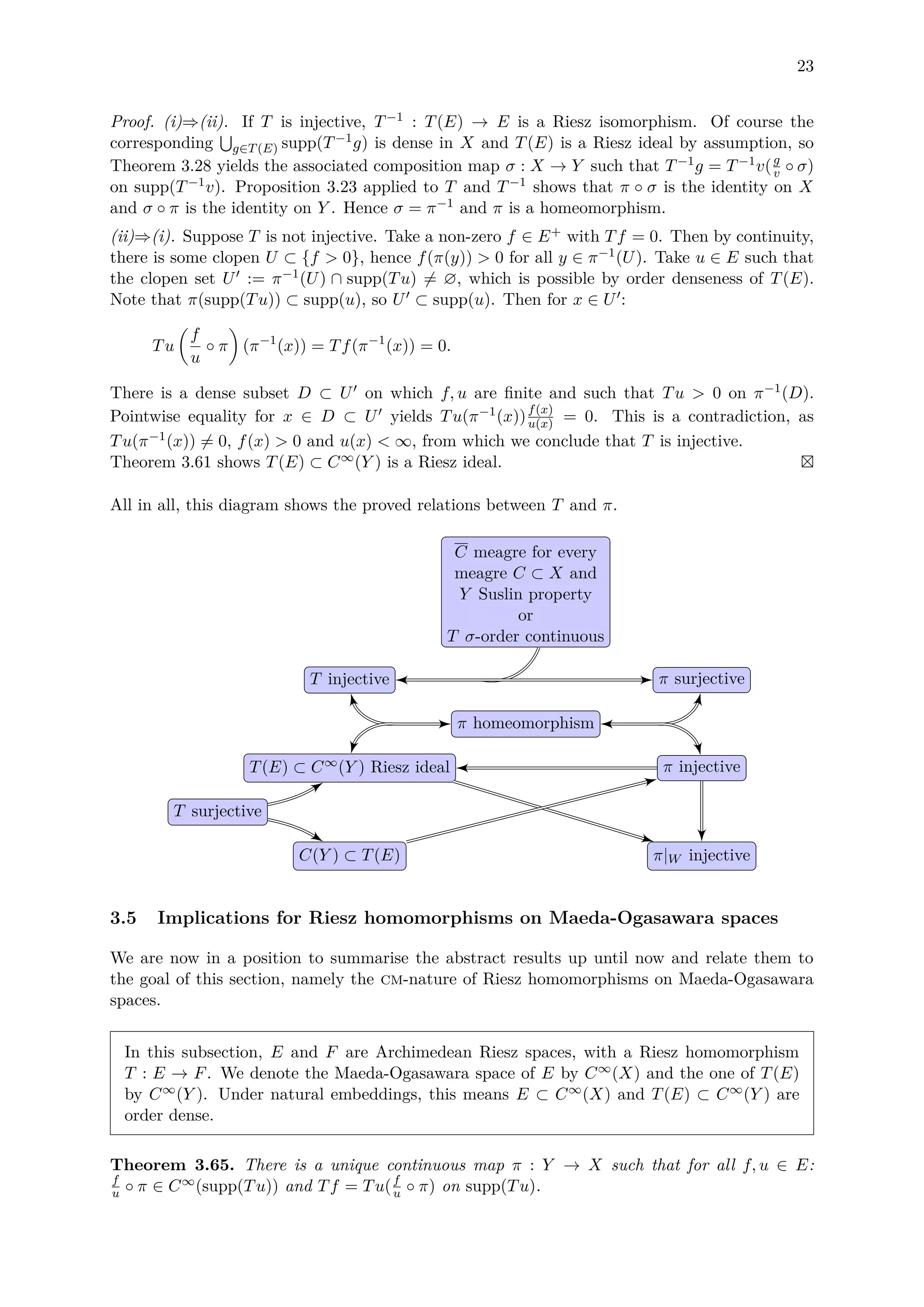
![24
Proof. Corollary 3.6 yields an extension T : E → C∞(Y ) of T to the ideal E generated by E.
Now apply Theorem 3.28 to find a unique continuous π : Y → X such that f
u ◦π ∈ C∞(supp(Tu))
and Tf = Tu(f
u ◦ π) on supp(Tu) for all f, u ∈ E.
It is clear that Theorem 3.29 yields a similar result.
E T(E) F
C∞
(X) C∞
(Y )
T
order dense order dense
⊂
π
The figure shows the embeddings of E and its image under T in their respective Maeda-
Ogasawara spaces. For the rest of this subsection, let π be this unique associated composition
map of T. An immediate consequence is the following.
Corollary 3.66. Suppose there exists some u ∈ E such that supp(Tu) = Y . Then there is an
η := Tu ∈ C∞(Y ) such that for all f ∈ E: Tf = η(f
u ◦ π).
Proposition 3.67. If T is order continuous, there is an η ∈ C∞(Y ) such that for every f ∈ E:
f ◦ π ∈ C∞(Y ) and Tf = η(f ◦ π).
Proof. This is a simple consequence of Corollary 3.43.
Proposition 3.68. If E contains a weak unit and T is σ-order continuous, there is an η ∈
C∞(Y ) such that for every f ∈ E: f ◦ π ∈ C∞(Y ) and Tf = η(f ◦ π).
Proof. As E contains a weak unit, we can embed E ⊂ C∞(X) such that 1X ∈ E. Then σ-
order continuity implies supp(T1X) = W = Y , so we define η := T1X and by Theorem 3.65:
f ◦ π ∈ C∞(Y ) and Tf = T1X( f
1X
◦ π) = η(f ◦ π).
If E is Dedekind complete, we extend Theorem 3.65.
Proposition 3.69. Suppose E is Dedekind complete. If T is σ-order continuous, then for all
f, g ∈ E: Tg(f ◦ π) = Tf(g ◦ π) on supp(Tf) ∩ supp(Tg).
Proof. E is Dedekind complete, so E ⊂ C∞(X) is a Riesz ideal by Corollary 2.24. Hence we
apply Proposition 3.37 and Theorem 3.35, yielding the desired result.
Remark 3.70. Although these results are applicable to the Maeda-Ogasawara spaces of all
Archimedean Riesz spaces E and F, the direct implications for the original spaces are unclear,
due to the pointwise nature of all prior statements. This is hard to describe in general, but in
the next section we explore an application.
3.6 Application to spaces of measurable functions
At this point, we are interested in how the cm-nature of Riesz homomorphisms on the embedding
of an Archimedean Riesz space in its Maeda-Ogasawara space translates to the original space.
For this, we consider equivalence classes of measurable functions. In this subsection, we come
back to the relation between this thesis and [21].
Definition 3.71. A σ-finite measure space consists of a set Ω, a σ-algebra A of Ω, called the
measureable sets, and a non-negative measure µ : A → R+, with the property that there exists
a countable subset A ⊂ A with µ(A) < ∞ for all A ∈ A and Ω = A .](https://image.slidesharecdn.com/7a110103-c215-45ff-8349-ca9740682412-160901090557/75/Masterscriptie-T-Dings-4029100-30-2048.jpg)
![25
For the rest of this section, (Ω, A, µ) and (Λ, B, ν) are σ-finite measure spaces. We also drop
all our earlier defined notions of E, X, Y , and T.
Notation 3.72. Write L(Ω) := L(Ω, A, µ) for the space of measurable functions with subspaces
Lp(Ω) := Lp(Ω, A, µ) (1 ≤ p ≤ ∞) as usual. We denote the spaces of µ-equivalence classes by
M(Ω) and Lp(Ω), respectively.
Occasionally, we shall need to make the distinction between measurable functions and their
equivalence classes explicit. Instead of writing [f] ∈ M(Ω) for f ∈ L(Ω), we introduce the
following notation.
Notation 3.73. For an equivalence class of measurable functions f, we write f if any represen-
tative of that class can be substituted.
In the next theorems, we outline the situation for this subsection. A thorough treatment of the
subject, including the proofs and other technicalities, can be found in Chapter 17 of [12].
Theorem 3.74. There is an extremally disconnected compact Hausdorff space X with a multi-
plicative Riesz isomorphism ˆ· : M(Ω) → C∞(X), such that ˆ1Ω = 1X and:
(i) For A ∈ A, there is a unique clopen ˆA ⊂ X such that ˆ1A = 1 ˆA. Also, the other way
around, every clopen subset of X is ˆA for some A ∈ A. In particular, ˆA = ∅ if and only
if µ(A) = 0.
(ii) If f ∈ M(Ω) and A ∈ A, then f1A = ˆf1 ˆA.
(iii) For f, g ∈ M(Ω), we have:
• ˆf = 0 if and only if f = 0 µ-a.e.;
• ˆf ≤ ˆg if and only if f ≤ g µ-a.e.;
• |f| = | ˆf| and −f = − ˆf.
(iv) The restriction of ˆ· to L∞(Ω) is a multiplicative isometric Riesz isomorphism L∞(Ω) →
C(X).
C∞(X) is clearly the Maeda-Ogasawara space of M(Ω) and all its order dense subspaces.
Notation 3.75. For the sake of readability, we sometimes write [f]ˆ instead of ˆf.
Notation 3.76. For f, g : X → [−∞, ∞], we denote that {f = g} is meagre by f ≡ g. For
U, V ⊂ X, we write U ≡ V if 1U ≡ 1V .
Theorem 3.77. The collection of all U ⊂ X for which there is a clopen V such that V ≡ U
is a σ-algebra, obviously containing all clopen and all meagre sets. We denote this collection
by ˜A. Note that ˆA ∈ ˜A for all A ∈ A. Define ˜µ : ˜A → [0, ∞] by ˜µ( ˜A) := µ( ˆA), for ˜A ≡
ˆA. Then (X, ˜A, ˜µ) is a σ-finite measure space, the completion of (X, Clopen(X), ˜µ|Clopen(X)).
Furthermore, ˆ· : Lp(Ω) → Lp(X) := Lp(X, ˜A, ˜µ) is a Riesz isomorphism.
Corollary 3.78. In the above situation, where M(Ω) ∼= C∞(X), X has the Suslin property.
Proof. Suppose ˆC is an uncountable collection of disjoint clopen subsets of X and write C :=
{C | ˆC ∈ ˆC}. Let A ⊂ A be a countable subset such that µ(A) < ∞ for all A ∈ A and Ω = A .
For all A ∈ A and C ∈ C: µ(C ∩ A) ≤ µ(A). For every n ∈ N>0, we have
C ∈ C | µ(C ∩ A) > 1
n ≤ nµ(A),
which is finite because µ(A) is finite. Hence the total number of non-negligible sets in {C∩A | C ∈
C} is countable for every A ∈ A , so by countability of A , the total number of non-empty sets
in ˆC is countable.](https://image.slidesharecdn.com/7a110103-c215-45ff-8349-ca9740682412-160901090557/75/Masterscriptie-T-Dings-4029100-31-2048.jpg)
![26
From [15], we adopt the following terminology, for similar purposes as in [21].
Definition 3.79 (Rodriguez-Salinas). A set map τ : A → B is a ν-homomorphism if for every
sequence (An)n in A:
ν τ An τ(An) = 0 and ν τ An τ(An) = 0.
To be able to study composition operators, we need to connect set maps and measurable func-
tions. This lemma allows us to extend the obvious ‘composition’ with A-simple functions to
arbitrary elements of M(Ω).
Lemma 3.80 (Rodriguez-Salinas). Let τ : A → B be a set map. For a positive A-simple
function s := N
n=1 λn1An , we (symbolically) define a new A-simple function by
s ◦ τ−1
:=
N
n=1
λn1τ(An).
If τ is a ν-homomorphism, we extend this definition to any positive measurable function f ∈ M
by choosing a non-decreasing sequence of A-simple functions (fn)n such that n fn = f and
defining f ◦ τ−1 := n fn ◦ τ−1. This way, f → f ◦ τ−1 is well-defined, linear and order-
preserving.
3.6.1 Cm-operators on M(Ω)
To summarise, Theorems 3.74 and 3.77 provide a clear correspondence between the spaces
of measurable functions on (Ω, A, µ) and (Λ, B, ν) and extended continuous functions on the
extremally disconnected compact Hausdorff spaces X and Y . This allows us to apply the earlier
results of this section. We develop a statement similar to Theorem 3.28, which is in fact a more
general version of a result from [21] (viz. Remark 3.84), from which we first slightly alter Lemma
3.7.
Lemma 3.81. Let I(Ω) ⊂ M(Ω) be a Riesz subspace and T : I(Ω) → M(Λ) a σ-order continuous
Riesz homomorphism. Then τ : A → B given by A → {T1A > 0} is a ν-homomorphism.
Proof. The crucial step in the proof is the equality T( n 1An ) = n T1An for all sequences
(An)n in A, which is covered by the assumption that T is σ-order continuous:
τ( n An) = {T1
n
An
> 0}
= {T( n 1An ) > 0}
= { n T1An > 0}
= n{T1An > 0}
= n τ(An),
as desired.
Theorem 3.82. Let I(Ω) ⊂ M(Ω) be an order dense ideal and T : I(Ω) → M(Λ) an order
continuous Riesz homomorphism. Then there are σ : A → B and η ∈ M(Λ) such that Tf =
η(f ◦ σ−1) for every f ∈ I(Ω). In addition, σ(A) = {T1A > 0} for all A ∈ A, and σ is a
ν-homomorphism.
Proof. Write
J(Λ) := T(I(Ω));
I(X) := I(Ω) ⊂ C∞(X) ∼= M(Ω);
J(Y ) := J(Λ) ⊂ C∞(Y ) ∼= M(Λ).](https://image.slidesharecdn.com/7a110103-c215-45ff-8349-ca9740682412-160901090557/75/Masterscriptie-T-Dings-4029100-32-2048.jpg)
![27
Denote the natural σ-algebras in X and Y by ˜A and ˜B, respectively. I(X) is Dedekind complete
by Corollary 2.26, hence I(Ω) is. Applying Theorem 3.42 to T, we get an order continuous
extension ˜T : M(Ω) → M(Λ). Define ˜S : C∞(X) → C∞(Y ) by ˜S ˆf = ˜Tf and set ˆη :=
˜S1X. Order continuity ensures that supp(ˆη) = W, which allows us to assume order denseness
of J(Y ) ⊂ C∞(Y ) without loss of generality. Then by Theorem 3.28, there exists a unique
continuous π : Y → X such that ˜S ˆf = ˆη( ˆf ◦ π).
J(Ω) J(Λ)
M(Ω) M(Λ)
I(X) C∞
(X) C∞
(Y ) J(Y )
ˆ·
⊂
T
⊂
ˆ·
ˆ·
˜T
ˆ·
⊂
˜S
π
⊃
1
Considering π−1 as a map on ˆA, we have π−1( ˆA) ∈ ˆB. Via ˆ·, this yields σ : A → B by
σ(A) := π−1( ˆA). Then for A ∈ A:
T1A = ˜Sˆ1A = ˜S1 ˆA
= ˆη(1 ˆA ◦ π) = ˆη1π−1( ˆA)
= ˆη1σ(A)
= ˆηˆ1σ(A)
= ˆη[(1A ◦ σ−1)]ˆ = [η(1A ◦ σ−1)]ˆ.
We conclude T1A = η(1A ◦ σ−1) = η1σ(A). Observe that {η = 0} ⊂ {T1A = 0}, so {T1A >
0} = {1σ(A) = 0} = σ(A), as desired. The preceding lemma proves σ is a ν-homomorphism.
Lemma 3.80 allows us to extend f → η(f ◦ σ−1) to the whole I(Ω), completing the proof.
At first sight, it seems restrictive to impose order continuity of the Riesz homomorphism. How-
ever, there are natural ideals I(Ω) ⊂ M(Ω) for which every Riesz homomorphism T : I(Ω) →
M(Λ) is order continuous. As an example, we cite Corollary 3.6 from [21].
Proposition 3.83. Let (1 ≤ p < ∞). Every Riesz homomorphism T : Lp(Ω) → M(Λ) is order
continuous.
Remark 3.84. For Lp spaces, Theorem 3.82 is equivalent to Theorem 3.8 of [21]. Note that
this result is more general, as it for example applies to Lp for p < 1.
In view of Section 3.3.2, we can do more. Proposition 3.49 allows us to reformulate Theorem
3.82 in a slightly stronger way.
Theorem 3.85. Let I(Ω) ⊂ M(Ω) be an order dense ideal and let T : I(Ω) → M(Λ) be a
σ-order continuous Riesz homomorphism. Then there are a ν-homomorphism σ : A → B and
an η ∈ M(Λ) such that Tf = η(f ◦ σ−1) for every f ∈ I(Ω). Again, σ(A) = {T1A > 0}, which
is a ν-homomorphism.
Proof. We follow the proof of Theorem 3.82, in which T and ˜T are σ-order continuous this time.
Corollary 3.78 and Proposition 3.49 assure ˜T exists. By σ-order continuity, Lemma 3.37 proves
that supp(ˆη) = W and Lemma 3.81 implies that σ is a ν-homomorphism.
Although the Lp spaces for 1 ≤ p < ∞ are emphasised, L∞(Ω) is of course also an order dense
Riesz subspace of M(Ω). Hence Theorem 3.85 is applicable just as well. The major difference is
that not all Riesz homomorphisms on L∞ are order continuous, in contrast to Proposition 3.83.](https://image.slidesharecdn.com/7a110103-c215-45ff-8349-ca9740682412-160901090557/75/Masterscriptie-T-Dings-4029100-33-2048.jpg)
![28
Remark 3.86. Let us consider a Riesz homomorphism T : L∞(Ω) → M(Λ). We show that we
can not drop the assumption that T is σ-continuous, if we want to prove T is of a cm-form.
Following the proof of Theorem 3.82, part (iv) of Theorem 3.74 shows that 1X ∈ ˆL∞(Ω) =
C(X). Setting S ˆf := Tf, we define ˆη := S1X. Observe that 1X is a strong unit in C(X), so
W = supp(η) and there is no need to extend T to M(Ω). We find a continuous π : W → X10
such that S ˆf = ˆη( ˆf ◦ π). Again, this yields σ : A → B such that T1A = η(1A ◦ σ−1), where
σ(A) = {T1A > 0}. Up until this point, matters seem promising, but we observe that σ is
not necessarily a µ-homomorphism. That means Lemma 3.81 is not applicable to extend the
formula from simple to arbitrary measurable functions.
We have derived results resembling Theorem 2.11 for subspaces of measurable functions, but
the transferred associated composition map σ is defined on the σ-algebra, not pointwise. Of
course, one has to be careful with pointwise properties on measurable spaces. Even so, partially
inspired by the closing remarks in [21], in the next subsection we wonder whether any genuine
cm-properties can be established.
3.6.2 Set maps induced by point maps
In special cases, set maps on A are induced by point maps on the underlying space Ω. As already
mentioned, our starting point is the remark at the end of page 23 of [21], about the efforts of
Halmos and Von Neumann in [23] and [7]. Although these works do not seem to be directly
applicable, we find a helpful clue in [16].
Definition 3.87. A map σ : A → B is induced by a point map if there is a φ : Λ → Ω such that
σ(A) = φ−1(A) for every A ∈ A.
Definition 3.88. A two-valued measure on a σ-algebra A is a function m : A → {0, 1} such
that m(Ω) = 1 and m(A1 ∪A2) = m(A1)+m(A2) for any two disjoint Ai ∈ A. We call m trivial
if there is some ω ∈ Ω such that m(A) = 1 if and only if ω ∈ A.
Theorem 3.89 (Sikorski). Every ν-homomorphism σ : A → B is induced by a point map if and
only if every two-valued measure on Ω is trivial.
Lemma 3.90. If A is countably generated, every two-valued measure on A is trivial.
Proof. Suppose A is generated by A1, A2, . . . . For every n, either m(An) = 1 or m(Ac
n) = 1.
Define An to be An if m(An) = 1 and Ac
n if m(An) = 0, with A0 := An. Then m(A0) = 1,
hence A0 = ∅. Now take an arbitrary A ∈ A. For any ω0 ∈ A0, we have m(A) = 1 if and only
if ω0 ∈ A. Hence m is trivial.
Exploring these spaces further, we find Proposition 3.2 in [14] to be useful.
Definition 3.91. For a topological space X, we call the σ-algebra generated by the open sets
in X its Borel σ-algebra, and denote it by B(X).
Definition 3.92. A set map τ : A → B is measurable if τ−1(B) ⊂ A and exactly measurable if
τ−1(B) = A.
Proposition 3.93. A is countably generated if and only if there exists an exactly measurable
mapping τ : A → B({0, 1}N).
10
or Y → X, if we assume the image J(Λ) of T to be order dense in M(Λ)](https://image.slidesharecdn.com/7a110103-c215-45ff-8349-ca9740682412-160901090557/75/Masterscriptie-T-Dings-4029100-34-2048.jpg)


![31
4 Generalised cm-operators on C(X; E)
In multivariate analysis, one would like to study continuous functions of multiple variables by
focusing on one at a time. In the first part of this section, we study direct consequences of
Theorem 2.11 in this context. Later on, we will see that similar results hold in a more general
setting.
4.1 Riesz homomorphisms on C(X; C(Y ))
In this subsection, X, Y, Z are compact Hausdorff spaces. This allows us to directly apply
Lemma 2.10 and Theorem 2.11, with help of Theorem 8.20 from [13].
Theorem 4.1. For locally compact spaces A, B, C, the canonical map J : C(A × B; C) →
C(A; C(B; C)) given by f(x, y) → ˜f(x)(y) := f(x, y) is a homeomorphism (with respect to the
compact-open topologies).
In case C = R and all spaces are equipped with the sup-norm, it is obvious that J is a Riesz
isomorphism.
Notation 4.2. In C(X; C(Y )), we denote the function x → 1Y for every x by ˜1. Note that
J1X×Y = ˜1.
Lemma 4.3. Let T : C(X; C(Y )) → R be a Riesz homomorphism. Then there are x0 ∈ X,
y0 ∈ Y such that T ˜f = (T ˜1) ˜f(x0)(y0).
Proof. The space X × Y is compact and TJ : C(X × Y ) → R is a Riesz homomorphism, so
Lemma 2.10 yields (x0, y0) ∈ X×Y with T ˜f = TJf = (TJ1X×Y )f(x0, y0) = (T ˜1) ˜f(x0)(y0).
Corollary 4.4. Let T : C(X; C(Y )) → C(Z) be a Riesz homomorphism. Set η := T ˜1. Then
there is a map π : Z → X × Y , which is continuous on {η > 0}, such that T ˜f = η(f ◦ π).
Proof. This time we apply Theorem 2.11 to C(X × Y ), indeed leading to π : Z → X × Y
continuous on {η > 0} such that T ˜f = TJf = (TJ1X×Y )(f ◦ π) = η(f ◦ π).
Although C(X × Y ) ∼= C(X; C(Y )), the former is symmetric in X and Y , while the latter is
not. In view of the next section, we can rewrite the preceding as follows.
Corollary 4.5. Let T : C(X; C(Y )) → C(Z) be a Riesz homomorphism. Then there are
φ : Z → C(Y )∗ and π : Z → X such that T ˜f(z) = φ(z)( ˜f(π (z))). Moreover, φ is bounded and
weak* continuous, and π is continuous on {φ > 0}.
Proof. We have T ˜f(z) = T ˜1(z)f(π(z)), with π : Z → X × Y continuous on {T ˜1 > 0}. Now
set φ(z) := T ˜1(z)δπ2(z) and π (z) := π1(z), where πn represents the projection on the nth
coordinate. We immediately arrive at
T ˜f(z) = T ˜1(z)f(π(z)) = T ˜1(z) ˜f(π1(z))(π2(z)) = T ˜1(z)δπ2(z)
˜f(π1(z)) = φ(z)( ˜f(π (z))). (6)
Continuity of π follows from continuity of π, as {φ > 0} = {T ˜1 > 0}. Boundedness of φ
is immediate from boundedness of T: ||φ(z)||C(Y )∗ = ||T ˜1δπ2(z)||C(Y )∗ ≤ ||T||op. For fixed
g ∈ C(Y ): φ(z)(g) = T ˜1(z)g(π2(z)), which is continuous in z by continuity of T ˜1, g and π.
Remark 4.6. φ is in general not continuous with respect to the operator norm:
||φ(z) − φ(z )||C(Y )∗ = sup
||g||∞≤1
|T ˜1(z)δπ2(z)(g) − T ˜1(z )δπ2(z )(g)| = 2||T||op,
if π2(z) = π2(z ).](https://image.slidesharecdn.com/7a110103-c215-45ff-8349-ca9740682412-160901090557/75/Masterscriptie-T-Dings-4029100-37-2048.jpg)
![32
4.2 Riesz homomorphisms on C(X; E)
To generalise this idea, we replace C(Y ) by a space E, for which we introduce a more generic
concept. Furthermore, we explore a larger class of spaces than only compact ones.
Definition 4.7. A Banach lattice is a Riesz space which is also a complete normed space, with
the property that |f| ≤ |g| implies ||f|| ≤ ||g||.
If Y is compact, then C(Y ) with the sup-norm is a Banach lattice.
Definition 4.8. A topological space is realcompact if it can be embedded homeomorphically
as a closed subset in some Cartesian power of the real numbers, equipped with the product
topology.
Every compact space is also realcompact.
It turns out that realcompactness is precisely what we need, so throughout this subsection,
let X, Z be realcompact Hausdorff spaces and E a Banach lattice. If dim(E) = 0, we trivially
have C(X; E) ∼= {0}, so we assume dim(E) ≥ 1.
Turning back once again to the formulation of Lemma 2.10 and Theorem 2.11, we cite [4] for a
generalised version of the lemma.
Lemma 4.9. Let φ : C(X) → R be a Riesz homomorphism. Then φ(f) = φ(1)f(x0) for some
x0 ∈ X.
The proof of Theorem 2.11 in [3] does not make use of compactness, so we may equally apply
the result to continuous functions on realcompact spaces.
Corollary 4.10. Let T : C(X) → C(Z) be a Riesz homomorphism. Then there are η ∈ C(Z)
and π : Z → X continuous on {η > 0} satisfying Tf = η(f ◦ π) for all f ∈ C(X).
The lemma allows us to generalise Lemma 2.10.
Proposition 4.11. Let T : C(X; E) → R be a Riesz homomorphism. Then there are x0 ∈ X
and a Riesz homomorphism φ : E → R such that Tf = φ(f(x0)) for all f ∈ C(X; E).
Proof. Let g ∈ C(X; E)+ and consider the map Sg : u → T(ug) from C(X) to R. This is a
Riesz homomorphism, hence there is an xg ∈ X such that Sgu = Sg1Xu(xg) = Tg · u(xg). For
g ∈ C(X; E)+ the preceding yields xg ∈ X such that Sg = Tg · u(xg ). Then Sg + Sg = Sg+g ,
so finally xg = xg = xg+g . We conclude that there exists an x0 ∈ X such that T(ug) = Tg·u(x0)
for all g ∈ C(X; E), u ∈ C(X).
Now choose f ∈ C(X; E) arbitrarily and define
u(x) := ||f(x)||E
g(x) :=
f(x)
√
||f(x)||E
if f(x) = 0
0 if f(x) = 0,
so u ∈ C(X), g ∈ C(X; E) and f = ug. First, assuming f(x0) = 0, we have u(x0) = 0 and
Tf = T(ug) = Tg · u(x0) = 0. Now suppose f(x0) = f (x0) for some f ∈ C(X; E). Then
Tf − Tf = T(f − f ) = 0 because (f − f )(x0) = 0, so Tf = Tf . We conclude that Tf only
depends on f(x0), so we define φ : E → R by φ(e) := T(x → e). This φ is a Riesz homomorphism
because T is, and we conclude Tf = φ(f(x0)) for all f ∈ C(X; E).](https://image.slidesharecdn.com/7a110103-c215-45ff-8349-ca9740682412-160901090557/75/Masterscriptie-T-Dings-4029100-38-2048.jpg)

![35
5 Discussion
The results of this thesis indeed indicate that every Riesz homomorphism between Archimedean
Riesz spaces is, in the sense of the embedding in its Maeda-Ogasawara space, a generalised cm-
operator. The argument is based on and inspired by Theorem 2.11, ensuring that our results
yield the same expression in the degenerate case of a space of ordinary continuous functions.
Our work fits in the line of generalisations to for example spaces of Lipschitz functions in [10]
or spaces of continuous functions on locally compact Hausdorff spaces in [9]. Regarding Section
4, we mention that [8] contains related work.
For the sake of readability, let us again refer to the setting as considered in Section 3.5 and
shown in the figure.
E T(E) F
C∞
(X) C∞
(Y )
T
order dense order dense
⊂
π
The Maeda-Ogasawara Theorem provides a description in terms of functions of all Archimedean
Riesz spaces, making the main result of thesis, stated in its purest form in Theorem 3.65,
widely applicable. At the same time, the explicit construction is not so easy to manipulate,12
which makes it hard to see how pointwise results for the embeddings of E and T(E) in their
Maeda-Ogasawara spaces translate to the original situation. In the last part of Section 3.2, we
nonetheless succeed in proving general statements without any pointwise character.
An obvious way to evade this problem is to study a setting in which a clear description of the
Maeda-Ogasawara space is available. Partly inspired by the second part of [21], Section 3.6
explores the implications of the developed theory for spaces of measurable functions, and in
particular for the familiar Lp spaces. Although one should always be careful with pointwise
descriptions in this situation, Theorems 3.85 and 3.94 provide clear results. It is interesting to
see that this detour extends the results of [21].
Let us mention some challenges, that might indicate interesting directions for further research.
In the classical case of ordinary continuous functions on X and Y , every continuous map from
Y to X induces a composition operator. The notorious complication here is that not every such
map is the associated composition map of a Riesz homomorphism from C∞(X) to C∞(Y ). It is
unclear how to describe the exact conditions for its behaviour on meagre subsets the map has to
satisfy to induce a well-defined (generalised) composition operator. It is generally not possible
for every meagre subset of X to find an element of C∞(X) that is infinite on that particular
subset, indicating that the properties of these Maeda-Ogasawara spaces and their subspaces are
at moments rather counter-intuitive.
The examples presented in this thesis – most notably in Section 3.6, but also the different studies
of C∞(βN) – indicate that most practical situations are in one way or another neater than
the general setting. When either the homomorphism or the spaces satisfy certain countability
restrictions, our results collapse into more straightforward expressions, the best example being
Theorem 3.43: if T is order continuous, we retrieve the ordinary cm-form. Stated the other
way around, this means that it is not so easy to find non-trivial examples of the most general
situation. This also relates to the open end in Section 3.4, explained in Remark 3.56: to construct
an example in which T is not injective while π is surjective, T cannot be σ-order continuous, and
X and Y must be sufficiently large to not have the Suslin property.13 It would be interesting to,
12
The extremally disconnected space X contains the prime ideals in the Boolean algebra of the bands of E,
equipped with the hull-kernel topology.
13
thereby excluding the measurable functions on a σ-finite measure space, as studied in Section 3.6](https://image.slidesharecdn.com/7a110103-c215-45ff-8349-ca9740682412-160901090557/75/Masterscriptie-T-Dings-4029100-41-2048.jpg)

![37
6 Samenvatting
Een wiskundige structuur wordt gedefinieerd door de eigenschappen die ze heeft. In deze scrip-
tie worden zogenaamde Rieszruimten14 bestudeerd, welke twee wiskundige concepten vereni-
gen. Ten eerste kennen we de vectorruimte, waarvan de elementen onderling kunnen worden
opgeteld en vermenigvuldigd met een re¨eel getal. Vervolgens zijn er tralies,15 waarin een orde-
ning gedefinieerd is zodat er voor elke twee elementen een uniek supremum en infimum bestaat.16
Een Rieszruimte is een vectorruimte die ook een tralie is. Het platte vlak, dat we met R2 aan-
duiden, is een eenvoudig voorbeeld. Optelling werkt puntsgewijs en als ordening nemen we
(x1, x2) ≤ (y1, y2) als x1 ≤ y1 en x2 ≤ y2.
In het linkerdiagram zien we de som (−1, 2)+(3, 1) = (2, 3) en de scalaire vermenigvuldiging
2 · (3, 1) = (6, 2). Aan de rechterkant is het supremum (3, 2) = (−1, 2) ∨ (3, 1) aangegeven.
Zo is R2 een vectorruimte en een tralie. In deze scriptie kijken we echter op een ietwat andere
manier naar de genoemde eigenschappen. Laten we bijvoorbeeld continue functies op het interval
[0, 1] bekijken, genoteerd als C[0, 1]. Zo’n functie f neemt een getal x tussen 0 en 1 als input, en
geeft een re¨eel getal f(x) terug. We schrijven: voor x ∈ [0, 1] hebben we f(x) ∈ R.17 Continu¨ıteit
houdt (informeel gesproken) in dat de grafiek van de functie geen onderbrekingen heeft, dus te
tekenen is zonder de pen van het papier te halen. We zeggen dat f ≤ g als f overal onder g
ligt, dus als f(x) ≤ g(x) voor elke x ∈ [0, 1]. Zulke functies kunnen we puntsgewijs optellen, dus
(f + g)(x) = f(x) + g(x). Ook kunnen we een functie vermenigvuldigen met een getal, eveneens
puntsgewijs. Tot slot heeft elk paar functies altijd een uniek supremum en infimum.
De twee functies f(x) = 9x2 − 10x + 1 en g(x) = x − 1
2 zijn links en in het midden geplot,
in het midden vergezeld door de som f + g en 2 · g. Helemaal rechts zien we het supremum
f ∨ g en infimum f ∧ g, waarvan de waarde voor elke x gegeven wordt door respectievelijk
het maximum en minimum van f(x) en g(x).
14
vernoemd naar de Hongaarse wiskundige Frigyes Riesz (1880-1956)
15
ook wel roosters genoemd
16
Het supremum van twee elementen x en y is het kleinste element dat groter is dan zowel x als y. We schrijven
x ∨ y. Op dezelfde manier is het infimum x ∧ y het grootste element dat kleiner is dan x en y.
17
Het symbool ∈ staat voor ‘is een element van’, dus x ∈ [0, 1] betekent dat 0 ≤ x ≤ 1. Als we de randpunten
niet toestaan schrijven we x ∈ (0, 1), dus dan 0 < x < 1.](https://image.slidesharecdn.com/7a110103-c215-45ff-8349-ca9740682412-160901090557/75/Masterscriptie-T-Dings-4029100-43-2048.jpg)
![38
Zo is C[0, 1] dus een Rieszruimte. Met behulp van deze begrippen kunnen we ook het positieve
en negatieve deel van een functie bekijken, waarvoor we f+ en f− schrijven. Uit de diagrammen
is duidelijk dat f = f+ − f−, verder defini¨eren we de absolute waarde van f als |f| = f+ + f−.
Links zien we dezelfde f en g; in het midden het positieve deel f+ en het negatieve deel g−;
rechts de absolute waarden |f| en |g|.
Nu is het interessant om naar afbeeldingen tussen functieruimten te kijken. Zo’n afbeelding
beeldt elke functie in de beginruimte af op een functie in de doelruimte.
Om dit concept te verduidelijken, bekijken we twee voorbeelden van afbeeldingen van C[0, 1]
naar zichzelf. De eerste is de vermenigvuldiging met een positieve functie,18 laten we zeggen
met h(x) = 2x2 − 1
4x + 1
4. We noteren de afbeelding daarom met Vh. Voor elke functie in
C[0, 1], bijvoorbeeld voor f van zojuist, hebben we dus Vhf = hf. Een kleine rekensom leert
dat Vhf(x) = h(x) · f(x) = 18x4 − 221
4x3 + 73
4x2 − 27
8 + 3
8. Zo hebben we voor elke functie in
C[0, 1] een beeld onder Vh in C[0, 1].
Het tweede voorbeeld is de samenstelling met een translatie. We noemen deze S. Hiervoor
nemen we een afbeelding van [0, 1] naar [0, 1], bijvoorbeeld π(x) = 1 − x, en defini¨eren we
Sf(x) = f(π(x)) = f(1 − x) = 9x2 − 8x + 1
2. Het beeld van f is dus de samenstelling van f met
π, dezelfde functie maar dan gespiegeld in de verticale lijn x = 1
2.
Links en rechts zien we kopie¨en van C[0, 1]: de afbeeldingen Vh en S sturen de functie f
links (samen geplot met de functie h) naar Vhf = hf en Sf = f(1 − x) rechts. Merk op dat
f en Sf elkaar spiegelbeeld zijn ten opzichte van de verticale lijn x = 1
2.
Vh,S
We kunnen vermenigvuldiging en samenstelling natuurlijk ook combineren in ´e´en afbeelding,
door een functie h eerst samen te stellen met π en dan te vermenigvuldigen met g. Laten we
deze afbeelding T noemen, dus Tf(x) = g(x)f(π(x)) = g(x)f(1 − x). Als we T beter bekijken,
is er een aantal zaken opmerkelijk te noemen. Wat eenvoudig rekenwerk wijst uit dat het niet
uitmaakt of we twee functies eerst optellen en dan via T afbeelden op de rechterkopie van C[0, 1],
of dat we juist eerst T toepassen en daarna optellen. Idem dito voor het nemen van suprema of
infima: we kunnen eerst f ∨ h uitrekenen en in T stoppen, maar ook eerst de beelden bekijken
en daarvan het supremum nemen.
18
dus een functie die overal boven de horizontale as ligt](https://image.slidesharecdn.com/7a110103-c215-45ff-8349-ca9740682412-160901090557/75/Masterscriptie-T-Dings-4029100-44-2048.jpg)
![39
Opnieuw twee keer C[0, 1]: links de functies f, h en f + h; rechts de beelden Tf, Th en
T(f + h).
T
We concluderen:
(i) T(f + h) = Tf + Th;
(ii) T(2 · f) = 2 · Tf (en ook voor elk ander re¨eel getal natuurlijk);
(iii) T(f ∨ h) = Tf ∨ Th;
(iv) T(f ∧ h) = Tf ∧ Th.
Deze afbeelding behoudt dus de volledige structuur van de Rieszruimte. Afbeeldingen die de
structuur van de ruimte waarop ze werken behouden, worden in het algemeen homomorfismen
genoemd: T is dus een Rieszhomomorfisme.
We komen nu bij het klassieke resultaat dat als inspiratie en basis voor deze scriptie dient. Zoals
gezegd is een afbeelding een Rieszhomomorfisme als zowel de sommen van functies als de orde-
ning op de ruimte behouden blijft. We hebben het voorbeeldhomomorfisme T geconstrueerd uit
een vermenigvuldiging met g (die we vanaf nu η noemen, om hem te onderscheiden van andere
elementen van C[0, 1]) en een samenstelling met π. We schrijven hiervoor Tf = η(f ◦ π) en noe-
men zo’n afbeelding een samenstellings-vermenigvuldigingsoperator (composition multiplication
operator, wat we afkorten tot cm-operator). De stelling waarop we voortbouwen zegt dat elk
Rieszhomomorfisme tussen twee ruimten van continue functies een cm-operator is, dus bestaat
uit een vermenigvuldiging en een samenstelling. Om te bepalen welke vermenigvuldigingsfunctie
er bij T hoort, bekijken we de constante functie die overal de waarde 1 heeft. We noteren die
met 1. Het blijkt dat T1 = η, dus het beeld van 1 is de functie die we zoeken.
C[0, 1] C[0, 1] T1 =: ηT
π
Het doel van deze scriptie is om te laten zien dat een vergelijkbare formulering werkt voor een
vele grotere klasse van Rieszruimten, dus niet alleen voor continue functies. Teneinde van C[0, 1]
in de context van deze scriptie te geraken, moeten we twee zaken aanpassen. Om te beginnen
staan we de functies toe de waarden oneindig en min oneindig19 aan te nemen. Dit mag echter
alleen op een ‘verwaarloosbaar’ stukje, dus bijvoorbeeld in ´e´en enkel punt. De ruimte van deze
uitgebreide continue functies noteren we met C∞[0, 1]. Belangrijke consequentie hiervan is dat
1 geen sterke eenheid meer is: voor een functie uit f ∈ C[0, 1] is er altijd een re¨eel getal n te
vinden waarvoor n · 1 ≥ f (bijvoorbeeld de waarde van f in zijn hoogste punt), maar als f
ergens de waarde oneindig heeft kan dat niet.
19
geschreven als ∞ en −∞](https://image.slidesharecdn.com/7a110103-c215-45ff-8349-ca9740682412-160901090557/75/Masterscriptie-T-Dings-4029100-45-2048.jpg)
![40
Voor een functie j ∈ C[0, 1] met j(1
2) = ∞ zien we door de plots van 1, 2 · 1 en 3 · 1 dat er
geen n ∈ R is waarvoor j ≤ n · 1.
Om er ondanks deze verandering voor te zorgen dat zo’n ruimte van uitgebreide continue functies
een Rieszruimte is (dus een vectorruimte en een tralie), moeten we de ruimte waarop we de
functies hebben gedefinieerd aanpassen. In plaats van het interval [0, 1] gaan we over op ruimtes
met een bijzondere eigenschap. In principe is daarin geen begrip van afstanden tussen punten,
maar we hebben wel omgevingen die ‘steeds nauwer’ om een punt liggen. Dan spreken we
informeel van ‘balletjes’ en ‘bolletjes’ om een punt, om aan te duiden of we de rand van de
verzameling wel of niet meenemen – zie ook voetnoot 17. In [0, 1] (waar wel een natuurlijk
afstandsbegrip is) is het balletje met straal 1
4 rond 1
2 bijvoorbeeld het interval [1
4, 3
4], dus inclusief
de randpunten 1
4 en 3
4, terwijl het corresponderende bolletje het interval (1
4, 3
4) is, zonder rand.
We noemen een ruimte extremaal onsamenhangend als voor elk tweetal bolletjes zonder overlap,
de bijbehorende balletjes ook geen elementen gemeen hebben. Merk meteen op dat [0, 1] dus
niet extremaal onsamenhangend is: de bolletjes (0, 1
2) en (1
2, 1) zijn disjunct, maar 1
2 zit in zowel
[0, 1
2] als [1
2, 1]. Informeel gesproken bestaat een extremaal onsamenhangende ruimte dus, zoals
de naam al aangeeft, uit onsamenhangende eilandjes die op een abstracte manier toch dicht bij
elkaar liggen.
Met al deze achtergrondkennis komen we terug op de eerder genoemde stelling. In deze scriptie
wordt beschreven op welke manier de theorie over cm-operatoren tussen ruimten van continue
functies kan worden gegeneraliseerd naar ruimten van uitgebreide continue functies. We bekijken
daarvoor niet per se de hele functieruimte, maar een deel ervan. Dat betekent dat we [0, 1]
inruilen voor X en Y , die beide extremaal onsamenhangend zijn. Dan nemen we een deelruimte
E van C∞(X),20 met een Rieszhomomorfisme T van E naar C∞(Y ). Het blijkt dat eenzelfde
formulering mogelijk is, dus met een afbeelding π van Y naar X, maar dat we geen eenduidige
functie η kunnen vinden zoals eerder.
E C∞
(Y )
C∞
(X)
T
⊂
π
Die η was gelijk aan het beeld van 1 onder T, maar omdat 1 geen sterke eenheid is, geeft
dat in deze situatie geen volledige beschrijving. Stel dat y ∈ Y waarvoor T1(y) = 0: dan
geldt Tf(y) = 0 voor elke begrensde f,21 maar niet voor elke f ∈ C∞(Y ). We moeten dus op
verschillende gebieden in Y verschillende vermenigvuldigingselementen toestaan, wat leidt tot
de formule Tf = Tu(f
u ◦ π) voor elk element u ∈ E. Met andere woorden: we vermenigvuldigen
20
Als A een deel van B is, schrijven we A ⊂ B.
21
want dan is er een getal n zodanig dat f ≤ n · 1, dus Tf(y) ≤ T(n · 1)(y) = n · T1(y) = n · 0 = 0](https://image.slidesharecdn.com/7a110103-c215-45ff-8349-ca9740682412-160901090557/75/Masterscriptie-T-Dings-4029100-46-2048.jpg)


![44
References
[1] C.D. Aliprantis and O. Burkinshaw. Locally solid Riesz spaces. Academic Press New York,
1978.
[2] C.D. Aliprantis and O. Burkinshaw. Locally solid Riesz spaces with applications to eco-
nomics. American Mathematical Society, 2003.
[3] C.D. Aliprantis and O. Burkinshaw. Positive operators. Springer, 2006.
[4] K. Boulabiar. Characters on C(X). Canadian Mathematics Bulletin, pages 7–8, 2014.
[5] E. de Jonge and A.C.M. van Rooij. Introduction to Riesz spaces. Mathematical Centre
Amsterdam, 1977.
[6] L. Gillman and M. Jerison. Rings of continuous functions. D. van Nostrand Company, Inc.,
1960.
[7] P.R. Halmos and J. von Neumann. Operator methods in classical mechanics II. Annals of
Mathematics, pages 332–350, 1942.
[8] J.E. Jamison and M. Rajagopalan. Weighted composition operator on C(X, E). Journal of
Operator Theory, pages 307–317, 1988.
[9] J.S. Jeang and N.C. Wong. Weighted composition operators of C0(X)’s. Mathematical
Analysis and Applications, pages 981–993, 1996.
[10] A. Jim´enez-Vargas and M. Villegas-Vallecillos. Linear isometries between spaces of vector-
valued Lipschitz functions. Proceedings of the American Mathematical Society, pages 1381–
1388, 2009.
[11] W.A.J. Luxemburg and A.C. Zaanen. Riesz spaces I. North-Holland Publishing Company,
1971.
[12] W.A.J. Luxemburg and A.C. Zaanen. Riesz spaces II. North-Holland Publishing Company,
1983.
[13] M. Manetti. Topology. Springer, 2015.
[14] C. Preston. Some notes on standard Borel and related spaces. Mathematical Proceedings,
2008.
[15] B. Rodr´ıguez-Salinas. On lattice homomorphisms on K¨othe function spaces. Reviews of the
Royal Academy of Sciences, Spain, pages 221–225, 1999.
[16] R. Sikorski. On the inducing of homomorphisms by mappings. Proceedings of the Polish
Mathematical Society, pages 7–22, 1947.
[17] R.M. Solovay and S. Tennenbaum. Iterated Cohen extensions and souslin’s problem. Annals
of Mathematics, pages 201–245, 1971.
[18] C.T. Tucker. Homomorphisms of Riesz spaces. Pacific Journal of Mathematics, pages
289–300, 1973.
[19] C.T. Tucker. Concerning σ-homomorphisms of Riesz spaces. Pacific Journal of Mathemat-
ics, pages 585–590, 1975.
[20] B. van Engelen. Lattice isomorphisms between Riesz spaces. Radboud University Nijmegen
(master’s thesis), 2015.](https://image.slidesharecdn.com/7a110103-c215-45ff-8349-ca9740682412-160901090557/75/Masterscriptie-T-Dings-4029100-50-2048.jpg)
![45
[21] H. van Imhoff. Composition multiplication operators on pre-Riesz spaces. Leiden University
(master’s thesis), 2014.
[22] A.C.M. van Rooij. Riesz spaces. Radboud University Nijmegen (lecture notes), 2011.
[23] J. von Neumann. Einige Satze uber messbare Abbildungen. Annals of Mathematics, pages
574–586, 1932.](https://image.slidesharecdn.com/7a110103-c215-45ff-8349-ca9740682412-160901090557/75/Masterscriptie-T-Dings-4029100-51-2048.jpg)