The document provides a comprehensive overview of communication systems, detailing the fundamentals of signals and systems, the elements involved in communication, and the various modes and media used for information exchange. It covers important topics such as modulation techniques, noise in communication systems, the benefits and disadvantages of electronic communication, and the distinction between analog and digital communications. Additionally, it discusses digital modulation techniques and their efficiency in transmitting information.


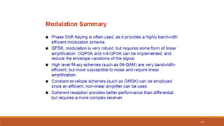
![Shannon’s Channel Capacity Theorem
R C = B * log2 {1 + (S / N)}
C – Capacity (bits/s), B – Bandwidth (Hz)
S – Signal Power (W), N – Noise Power (W)
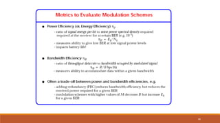
R/B log2 [ 1 + (Eb/ N0)(R/B) ]
( Eb - - Energy Per Bit, N0 – Noise Power Density )
Eb/N0 ( 2R/B -1 ) / (R/B) = ( 2 -1 ) /
Lim (B ) Eb / N0 = loge 2 = - 1.6 dB
Capacity of Communication Systems
128](https://image.slidesharecdn.com/presentation1communication-240507085616-81e2c7bd/85/Communication_System_presentation_Slides-pptx-128-320.jpg)
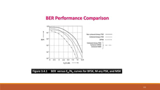
![-2 -1 6 12 18 24 30
16
8
4
2
1/2
1/4
M = 8
M = 16
M = 64
M = 4
MPSK
MQAM
Bandwidth
Limited
Region
Power
Limited
Region
Region for
R > C
Capacity Boundary
R = C
Shannon Limit
-1.59 dB
Eb / N0 (dB)
R/B ( b/s/Hz )
Bandwidth / Power Efficiency Plot
R/B log2 [ 1 + (Eb/ N0)(R/B) ]
129](https://image.slidesharecdn.com/presentation1communication-240507085616-81e2c7bd/85/Communication_System_presentation_Slides-pptx-129-320.jpg)


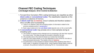


![Classification of signals (cont.)
For many cases, x[n] is obtained by sampling x(t) as:
x[n] = x(nT) , n =0,+1,+2,…
Are there any requirements for the sampling?
180](https://image.slidesharecdn.com/presentation1communication-240507085616-81e2c7bd/85/Communication_System_presentation_Slides-pptx-180-320.jpg)
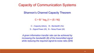
![Classification of signals (cont.)
2. Even and odd signals:
Even:
x(−t) = x(t)
x[−n] = x[n]
Odd:
x(−t) = −x(t)
x[−n] = −x[n]
Any signal x(t) can be expressed as
x(t) = xe(t) + xo(t) )
x(−t) = xe(t) − xo(t)
where xe(t) = 1/2(x(t) + x(−t)), xo(t) = 1/2(x(t) − x(−t))
181](https://image.slidesharecdn.com/presentation1communication-240507085616-81e2c7bd/85/Communication_System_presentation_Slides-pptx-181-320.jpg)
![Classification of signals (cont.)
3. Periodic and non-periodic signals:
CT signal: if x(t) = x(t + T), then x(t) is periodic.
Smallest T=Fundamental period: To
Fundamental frequency fo = 1/To (Hz or cycles/second)
Angular frequency: o = 2 /To (rad/seconds)
DT signal: if x[n] = x[n + N], then x[n] is periodic.
min(No): fundamental period
Fo = 1/No (cycles/sample)
=2 /N (rads/sample). If the unit of n is designated as dimensionless,
then is simply in radians.
Note: A sampled CT periodic signal may not be DT periodic.
Any Condition addition of two periodic CT signals, resultant
must be periodic signal ?
182](https://image.slidesharecdn.com/presentation1communication-240507085616-81e2c7bd/85/Communication_System_presentation_Slides-pptx-182-320.jpg)


![Classification of signals (cont.)
•DT signal x[n]:
Energy: E =
Power:
Energy signal: if 0 < E <
Power signal: if 0 < P <
2
x n
2
1
2 1
lim
N
N n N
x n
N
185](https://image.slidesharecdn.com/presentation1communication-240507085616-81e2c7bd/85/Communication_System_presentation_Slides-pptx-185-320.jpg)