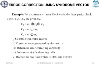
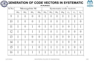
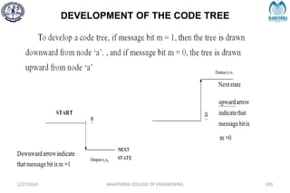
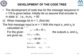
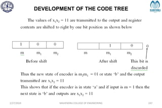
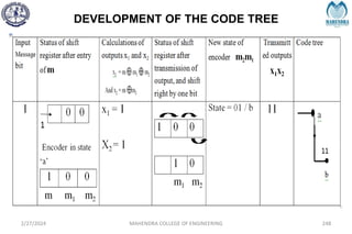
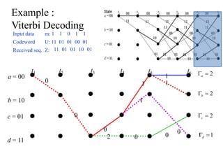
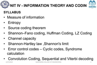
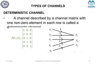
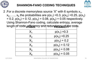
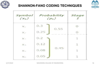
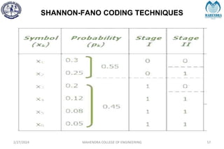
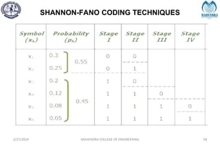
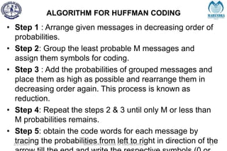
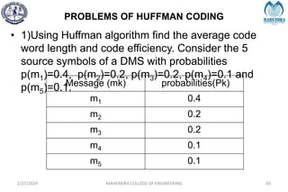
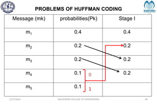
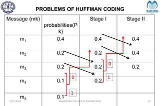
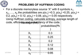
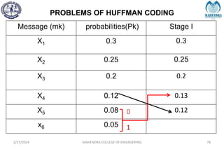
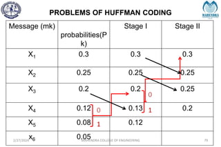
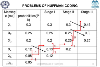
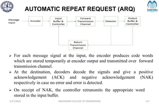
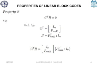
The document provides a comprehensive overview of information theory and coding, focusing on concepts such as measures of information, entropy, and various coding techniques like Shannon-Fano and Huffman coding. It discusses channel capacity and Shannon's theorem, which relate the maximum transmission rates of communication systems to their noise characteristics. Additionally, it outlines the principles of source coding and error control codes to ensure efficient and reliable transmission of information over communication channels.

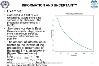


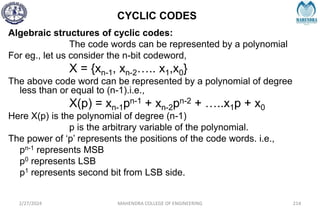
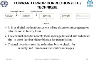
![IMPORTANT DEFINITIONS RELATED TO CODES
2/27/2024 MAHENDRA COLLEGE OF ENGINEERING 111
Hamming Distance:
The Hamming distance between two code words is equal
to the number of differences between them, e.g.,
1 0 0 1 1 0 1 1
1 1 0 1 0 0 1 0
Hamming distance = 3
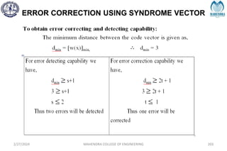
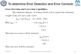
Minimum Distance dmin:
It is defined as the smallest Hamming distance between
any pair of code vectors in the code.
Hamming Weight of a Code Word [w(x)]:
It is defined as the number of non – zero elements in the
code word. It is denoted by w(x)
for eg: X= 01110101, then w(x) = 5](https://image.slidesharecdn.com/unitiv-240227101113-cffa9911/85/Communication-engineering-UNIT-IV-pptx-111-320.jpg)
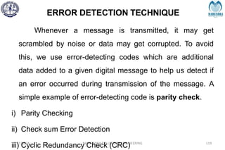


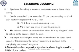
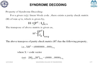
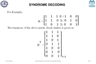
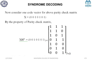
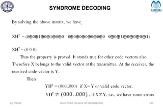
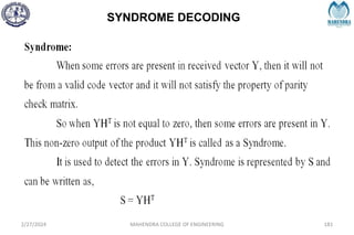
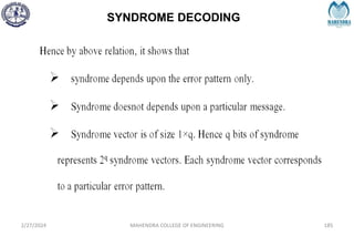
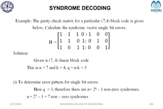
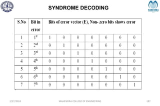
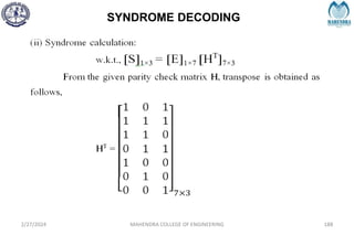
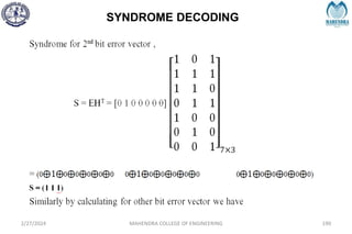
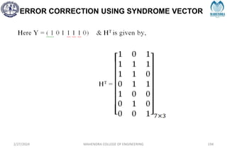
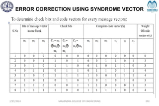
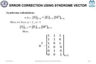
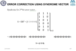
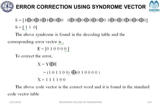
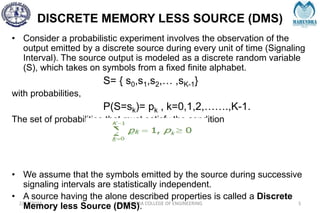
![SYNDROME DECODING
2/27/2024 MAHENDRA COLLEGE OF ENGINEERING 189
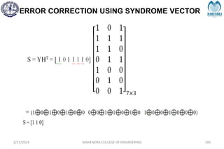
S = [1 0 1]](https://image.slidesharecdn.com/unitiv-240227101113-cffa9911/85/Communication-engineering-UNIT-IV-pptx-189-320.jpg)