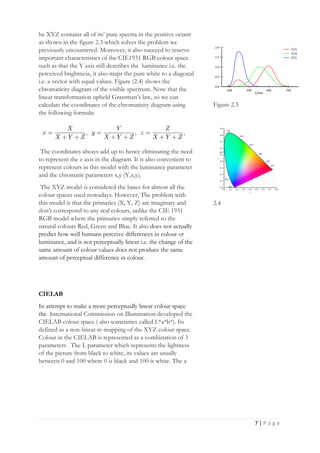
- Colour spaces are mathematical models that describe colours as tuples of numbers, usually three or four. They allow colours to be represented universally. - The CIE 1931 RGB and CIE 1931 XYZ colour spaces were the first developed based on colour matching experiments. XYZ defines colours in a positive space and preserves luminance (brightness). - Common colour spaces include CIE 1931 RGB, CIE 1931 XYZ, and CIELAB. They transform colours between perceptual and device-dependent representations.

1. COLOUR SPACES
Colour spaces and their use to computer vision
ABSTRACT
This paper is a simple introduction
to the use of colours in computer
vision, with a great focus on colour
spaces.
Khaled Nowara
Under the supervision of:
Eng. Mayar Al Fares
Eng. Mohamed Sabry

2. 1 | P a g e
Table of Contents
Computer vision 2
What is colour? 3
What is a colour space? 5
Types of colour space 6
CIE 1931 RGB 6
CIE 1931 XYZ 6
CIELAB 7
HSV 8
Appendix A 10
Appendix B 11
References 12

3. 2 | P a g e
Computer Vision
What is computer vision ?
Computer vision is the scientific field –it is actually an intersection
of a lot of different scientific fields as shown in figure 0.1- where
we try to extract information from digital images like depth
information, object identification, face recognition, etc. It is a field
of artificial intelligence where computers are trained to detect and
classify objects and react to what they see.
A little bit of history …
Computer vision dates back to 1966, specifically to a summer
undergraduate project with the goal to divide a vidisector picture
into regions such as
Likely objects
Likely backgrounds areas
Chaos.
It has been over 50 years and we haven’t still been able to solve the
problem of computer vision. Why is it so hard? Because what the
computer sees after all is an array of pixels, to extract useful
information out of these numbers is really complicated. Yet, we as
humans are subconsciously able to solve this problem in our own.
Our brains virtual cortex can easily do what we are trying to make
the computers do and definitely studying the brain can help us with
the Computer Vision dilemma.
Colour in Computer vision
Colour is one of the most important attributes of a picture when it comes
to computer vision, it plays a key role in a lot of application such as skin
detection, nude detection, and image segmentation. So it is important to
study the nature of colour and how is it modelled inside the computer
Figure 0.1

4. 3 | P a g e
What is colour ?
In order to study colour spaces an essential question arises.
What is colour? Colour is the entanglement of 2 properties.
First is the physical property determined by the difference in
wave length of electromagnetic waves that are in the
spectrum of visible light i.e. 370nm – 700nm. The second is
the psychological property of our visual experiences when we
look at stuff. Yes, in fact our perception of colour plays a
huge role in how we interpret the property colour. It is
important to be able to understand how living creatures –
humans especially- receive colours in order to be able to
represent, recreate and manipulate it.
Our visual system - or any visual system for that matter be it a
human, animal or even a computer- comes down to two
parts. Sensing and interpreting, as humans these roles are
filled by eyes and brains. We view the world around us
because of the way light goes through our eyes. Light rays
first passes the pupils and hit the retina. The retina is mainly
composed of 2 light sensitive types of cells, rods and cones –
named after their appearance under a microscope. In our
attempts in understanding our perception of colour we need
to focus on the cones. They are less sensitive, less numerous
than the rods but they are most useful at perceiving colours.
Cones come in three different types, characterized by a
unique response curve to different wave lengths of light
peaking at 440 nm, 530nm and 560 nm. Cones – as well as
rods- act as filters where the output can be interpreted as the
multiplication of each response curve integrated over all
wavelengths. Thus, encoding the information received into 3
numbers. The idea that we can represent the spectrum of
colours as a combination of 3 colours is the foundation of
systems that provides a consistent visual experience.
Figure 1.1
Figure 1.2

5. 4 | P a g e
It is worth mentioning that the our perception of light is not a
universal constant. For instance, we have no perception of
infra-red light mean while there are some species of fish and
snakes that are sensitive to infra-red radiation. In like manner,
dogs only have cones that are sensitive to yellow and blue
light only, along the same vein, shrimp mantis holds the
world record for the most number of cones with 12 different
kind of cones in their eyes. This information is important to
be able to understand that our perception of colours is more
of a personal and psychological experience i.e. my image of
blue in my mind can be the image of red in your mind.
In 1995 Wandell’s Foundation of Vision conducted
experiment that demonstrated people’s ability to recreate
colours by tuning 3 primary colours. The results showed that
the majority of people selected same colour tuning settings to
represent the test colours thus confirming trichromatic theory
of colour i.e. that three numbers are sufficient to encoding
colours. The theory dates back to Thomas Young’s writings
in the 1700s.
There are a lot of different ways to represent a certain colour.
If you recall from your childhood the famous colour
experiment where you create different colours from red,
green and blue lights. These are called additive primary
colours. Later on you might have learned about subtractive
primary colours i.e. cyan, magenta and pink. The ability to
represent a colour from a mixture of colours has nothing to
do with the wavelengths but rather the stimulus effects these
colours have on our cones.
In figure 1.3, you can see the additive primaries ( a ). You can
create the full range of the light spectrum by emitting these
primary colours i.e. if you are in room with no light and shine
a red and green lights you will get the yellow light and so on.
Meanwhile the subtractive primaries work as filters, you can
create the full range of light spectrum by reflecting white
light through these light filters.
Figure 1.3

6. 5 | P a g e
What is a colour space?
Now that we understand what colour is we can proceed to
define what colour space are. Simply they are the
mathematical model that describes a certain range of colours
as a tuples of numbers – normally three or four. A colour
space can be arbitrary or mathematically modelled.
Theoretically you can create any colour model to represent
any set of colours you want, however most commonly used
colour spaces can be transformed into a universally
understood system of colour interpretation.
Different colour spaces and their usage and their relation to
each other?
In 1920 Two experiments were conducted by W. Dave
Wright and john Guild. The subjects were viewed a test
colour and asked to match this colour by adjusting the
brightness of three primary colours. ( insert diagram ) Later in
1931 the Commission Internationale de l'Eclairage (French:
International Commission on Illumination – CIE ) developed
2 colour spaces i.e. The CIE 1931 RGB colour space and the
1931 XYZ colour space using this data. They were the first to
link the wavelengths of visible spectrums with the perceived
colours in our brain by performing colour matching
experiments. Using colour matching functions The CIE was
able to extract a numerical value for the luminosity of each
primary colour. The mathematical model of the colour
matching functions is as follows :
Appendix A is the implementation of the model in C
language.

7. 6 | P a g e
Types of colour spaces
CIE 1931 RGB
The RGB colour space is simply all the set of colours that can
be represented with different intensities of the colours red
green blue. The graph in the figure 2.1 above shows how you
can represent different colours of the spectrum using mixture
of the RGB lights corresponding to wave lengths 700nm,
546.1 nm and 435.8nm respectively. You can see that for a
certain range of spectra in the blue green range a negative
amount of red light is presents. That means this amount of
red has to be added to the test colour in order to get a colour
match. You can also think of the RGB colour space as the
R3 vector space, where red, green and blue corresponds to
the X, Y and Z axis respectively. The result will be a cube as
shown in figure (2.2). Note that there is a diagonal line where
R = G = B, this is called the grey line. Further details will be
discussed while discussing the HSV colour space. The
chromaticity of colours are defined in a trivial manner. It is
the ratio of the brightness of every primary colour with
respect to the other colours such that.
This is known as Grassman’s law
CIE 1931 XYZ
Due to the problems with the negative values in the CIE 1931
RGB colour space, the CIE developed a new colour space
called CIE 1931 XYZ or XYZ for short. The XYZ is just a
linear transformation of the CIE 1931 RGB colour space.
The transformation is given by the following formula:
Figure 2.1
Figure 2.2
T

8. 7 | P a g e
he XYZ contains all of its’ pure spectra in the positive octant
as shown in the figure 2.3 which solves the problem we
previously encountered. Moreover, it also succeed to reserve
important characteristics of the CIE1931 RGB colour space
such as that the Y axis still describes the luminance i.e. the
perceived brightness, it also maps the pure white to a diagonal
i.e. a vector with equal values. Figure (2.4) shows the
chromaticity diagram of the visible spectrum. Note that the
linear transformation upheld Grassman’s law, so we can
calculate the coordinates of the chromaticity diagram using
the following formula:
The coordinates always add up to hence eliminating the need
to represent the z axis in the diagram. It is also convenient to
represent colours in this model with the luminance parameter
and the chromatic parameters x,y (Y,x,y).
The XYZ model is considered the bases for almost all the
colour spaces used nowadays. However, The problem with
this model is that the primaries (X, Y, Z) are imaginary and
don’t correspond to any real colours, unlike the CIE 1931
RGB model where the primaries simply referred to the
natural colours Red, Green and Blue. It also does not actually
predict how well humans perceive differences in colour or
luminance, and is not perceptually linear i.e. the change of the
same amount of colour values does not produce the same
amount of perceptual difference in colour.
CIELAB
In attempt to make a more perceptually linear colour space
the International Commission on Illumination developed the
CIELAB colour space ( also sometimes called L*a*b*). Its
defined as a non-linear re-mapping of the XYZ colour space.
Colour in the CIELAB is represented as a combination of 3
parameters . The L parameter which represents the lightness
of the picture from black to white, its values are usually
between 0 and 100 where 0 is black and 100 is white. The a
Figure 2.3
2.4

9. 8 | P a g e
parameter that denotes the amount of red ( positive values of
a ) and green ( negative values of a ). The b parameter that
denotes the amount of yellow (positive value of b) and blue (
negative values of b). The mapping is defined as follows:
The CIELAB model is device independent meaning that it
defines colours regardless of how they are created or
displayed. Due to its perceptual linearity this colour space can
be used to make accurate colour balance corrections. Since
the CIELAB is a mathematical model, it is a public domain.
Hence, its used in a lot of different software like Adobe
Photoshop, Affinity lab, etc.
HSV
The HSV model is a cylindrical representation of the RGB
model where the grey line is taken as the center axis. It is used
along with the HSL to define the colours in a more intuitive
way that’s used by artists. HSV stands for Hue, Saturation and
Value. As shown in figure 2.6 the hue value is represented by
the angular dimension, the Saturation is represented by the
radial dimension and the value is the height dimension of the
cylinder. The transformation from the RGB model to the
HSV model is as follows, note that this is not a linear
transformation.
Figure 2.5
On the left is an CIELAB
enhanced colours
compared to the original
on the right
Figure 2.6

10. 9 | P a g e
The HSV model is used in photo editing and digital art
software because as mentioned earlier it more intuitive to
think of colours in terms of hue and saturation rather than
addition of primaries. It also contributes to high end graphics.
Moreover, this model is also used in colour recognition
software. Appendix B is a script in python language that
detects the colours Red, Green and Blue.
A lot of colour spaces were later developed like sRGB,
AdobeRGB and CMYK etc.. Each of these colour spaces
have different characteristics and of course different usage.
For instance the sRGB became standardized across the web
and computers. Meanwhile AdobeRGB is in professional and
higher end monitors as it has a wider gamut. The CMYK
(stands for cyan magenta yellow and black) is mainly used in
printing. In figure 2.8 you can see the different gaumats of
these colour spaces. As earlier mentioned most of the newer
colour models are a transformation from the XYZ model.
Figure 2.7
Adobe Photoshop using
the HSV model for colour
picking
Figure 2.8

11. 10 | P a g e
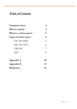
Appendix A
double gaussian(double x, double alpha, double mu, double sigma1,
double sigma2) {
double squareRoot = (x - mu)/(x < mu ? sigma1 : sigma2);
return alpha * exp( -(squareRoot * squareRoot)/2 );
}
void xyzFromWavelength(double* xyz, double wavelength) {
xyz[0] = gaussian(wavelength, 1.056, 5998, 379, 310)
+ gaussian(wavelength, 0.362, 4420, 160, 267)
+ gaussian(wavelength, -0.065, 5011, 204, 262);
xyz[1] = gaussian(wavelength, 0.821, 5688, 469, 405)
+ gaussian(wavelength, 0.286, 5309, 163, 311);
xyz[2] = gaussian(wavelength, 1.217, 4370, 118, 360)
+ gaussian(wavelength, 0.681, 4590, 260, 138);
}

12. 11 | P a g e
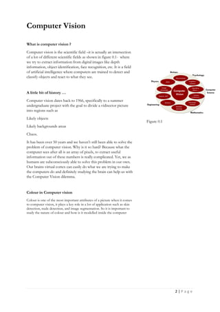
Appendix B
import cv2
import numpy as np
cap = cv2.VideoCapture(0)
while True:
_, frame = cap.read()
hsv_frame = cv2.cvtColor(frame, cv2.COLOR_BGR2HSV)
# Red color
low_red = np.array([161, 155, 84])
high_red = np.array([179, 255, 255])
red_mask = cv2.inRange(hsv_frame, low_red, high_red)
red = cv2.bitwise_and(frame, frame, mask=red_mask)
# Blue color
low_blue = np.array([94, 80, 2])
high_blue = np.array([126, 255, 255])
blue_mask = cv2.inRange(hsv_frame, low_blue, high_blue)
blue = cv2.bitwise_and(frame, frame, mask=blue_mask)
# Green color
low_green = np.array([25, 52, 72])
high_green = np.array([102, 255, 255])
green_mask = cv2.inRange(hsv_frame, low_green,
high_green)
green = cv2.bitwise_and(frame, frame, mask=green_mask)
cv2.imshow("Frame", frame)
cv2.imshow("Red", red)
cv2.imshow("Blue", blue)
cv2.imshow("Green", green)
cv2.imshow("Result", result)
key = cv2.waitKey(1)
if key == 27:
break
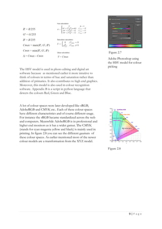
Description
First of all we need to import the
open CV and numpy modules.
Line 3 enables us to use the webcam
of the laptop and capture its frames.
Then for each colour we start by
defining the limits of the HSV
coordinates of the colour, then set a
new frame that shows only the
specified colours. Below you can see
the output of this code with the
original frame next to the masked one.

13. 12 | P a g e
References
HANDBOOK OF PATTERN RECOGNITION &
COMPUTER VISION by CH Chen, L F Pau & PS P Wan
Computer Vision: Algorithms and Applications by Richard Szeliski
Colour computer vision: fundamentals, applications and
challenges by Dr. Ignacio Molina-Conde, Depto. Tecnología
Electrónica Univ. of Málaga (Spain)
COMPUTER VISION : FOUNDATIONS AND
APPLICATIONS by Ranjay Krishna University of Stanford
wikipedia.org/CIE_1931_color_space
Khan academy.org/Colour science
Communicating pictures by David R. Bull
Total Colour Management in Textiles by B. Rigg
Vision Models for High Dynamic Range and Wide Colour Gamut
Imaging, by Marcelo Bertalmío
Pysource.com
Project mac, Artificial intelligence group 1966, MIT