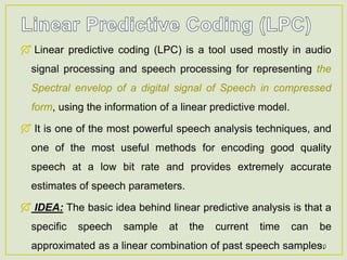
A MATLAB software
tool for SPEECH
analysis
1
2
About COLEA
Installation Instruction
Getting started & Guided Tour
Buttons in the MAIN COLEA WINDOW
PULL-DOWN MENUS
REFERENCES
CONCLUSION
3
• COLEA was originally developed in MATLAB 5.x, and is
actually a subset of a COchLEA Implants
Toolbox.
• It does not exploit the new features of MATLAB 7.x.
4
5
 System Requirement
₪ IBM compatible PC running Windows 95 (but we have windows 7/8 or XP)
₪ MATLAB ver. 5.x and MATLAB’s Signal Processing Toolbox (we used currently
7.10.x )
₪ Sound Card (any soundcard that runs in Windows, e.g., SoundBlaster)
₪ 700 Kbytes of disk space (we have free memory in Giga bytes)
 Installation Steps
₪ Download from http://www.utdallas.edu/~loizou/speech/colea.html
₪ PC/Windows
 After downloading the file ‘colea.zip’ to your PC, create a new directory/folder,
and unzip the file in that directory.
₪ Unix
 After downloading the file ‘colea.tar’, type: tar xvf colea.tar to un-tar the file.
This will automatically create a new directory called ‘colea’.
6
 After extract the files, you can see that COLEA can contains
several file formats by reading the extension of the file
 .WAV : Microsoft Windows audio files
 .WAV : NIST’s SPHERE format - new TIMIT format
 .ILS
 .ADF : CSRE software package format
 .ADC : old TIMIT database format
 .VOC : Creative Lab’s format
 The file extension is very important because each file format
has different header information.
 COLEA knows the file’s sampling frequency, the number of
samples, etc., by reading the header.
7
 Now illustrating some of COLEA’s features.
 Start the MATLAB.
 Open the colea.m file
 Run this file.
 click on change folder (if ASK!!!)
 Select the had.ils file.(from the COLEA extracted file
folder)
 Click on the waveform.
8
9
 This spectrum was obtained by performing a 12- pole
LPC analysis on the 10-msec speech segment
 So, when you click anywhere on the waveform using the
left mouse button, the program takes a 10-msec window
of the speech segment immediately after the cursor line,
and performs LPC analysis.
 You may change the size of the window, using the
Duration pull down option shown in the controls window
10
 Linear predictive coding (LPC) is a tool used mostly in audio
signal processing and speech processing for representing the
Spectral envelop of a digital signal of Speech in compressed
form, using the information of a linear predictive model.
 It is one of the most powerful speech analysis techniques, and
one of the most useful methods for encoding good quality
speech at a low bit rate and provides extremely accurate
estimates of speech parameters.
 IDEA: The basic idea behind linear predictive analysis is that a
specific speech sample at the current time can be
approximated as a linear combination of past speech samples.
11
 LPC order
 FFT Spectrum
 FFT size : you
have a choice on
the size of the FFT
 Overlay : If you
want to see the
FFT spectrum
overlaid on top of
the LPC spectrum
12
 Among other things, the controls window in Figure
2(CONTROLs) displays estimates of the formant
frequencies and formant amplitudes (in dB).
 The formant frequencies are computed by peak-picking
the LPC spectrum. To get accurate estimates of the
formant frequencies, one needs to choose the LPC order
properly depending on the sampling frequency.
 Increasing the LPC order to 18 will yield a better estimate
of the second and third formants
13
There are four pull-down menus in the LPC spectrum
window
 Print |Save | Label | Options
14
The Label menu is used for adding text or legends on the
figure or deleting existing text in the figure.
15
Options menu : Set Frequency Range
 This sub-menu is used for setting the frequency range.
16
Options menu : LPC analysis’
 this sub-menu is for setting a few options in LPC analysis
as well as FFT analysis [using (or not using) a pre-
emphasis FIR filter]
17
 Zoom in (Selected region) & Zoom Out
 Play: All & Sel (Selected interval is play)
18
19
 This tool is used for
comparing two waveforms
or two frames using either
time domain measures
(i.e., SNR) oror spectral domain measures (i.e., Itakura-Saito measure)
 To use this tool, you need first to load two waveforms where the
top is the approximated waveform and the bottom is the original
waveform.
The user has the option of making an overall (or global)
comparison between the two waveforms or a segmental (local)
20
 Overall : The two speech files are segmented in 10 msec
frames and the comparison is performed for each frame.
 At Cursor : To compare two particular speech segments
of the two files.
 The following distance measures are used :
 SNR : Signal-to-noise ratio
 CEP : Cepstrum
 WCEP : Weighted cepstrum (by a ramp)
 IS : Itakura-Saito
 LR : Likelihood ratio
 LLR : Log-likelihood ratio
 WLR : Weighted likelihood ratio
 WSM : Weighted slope distance metric (Klatt's)
21
 This tool is used for
adjusting the volume.
 There are three different modes:
 Autoscale (default) : The signal is automatically scaled
to the maximum value allowed by the hardware. In this
mode, you can not use the slider bar.
 No scale : In this mode the signal can be made louder
or softer by movin the slider bar.
 Absolute : In this mode, the signal is played as is. No
scaling is done. Moving the slider bar has no effect.
22
 Dual time-waveform and spectrogram displays
 Records speech directly into MATLAB NEW
 Displays time-aligned phonetic transcriptions
 Manual segmentation of speech waveforms - creates label
files which can be used to train speech recognition
systems
 Waveform editing - cutting, copying or pasting speech
segments
 Formant analysis - displays formant tracks of F1, F2 and
F3
 Pitch analysis
 Filter tool - filters speech signal at cut-off frequencies
specified by the user
 Comparison tool - compares two waveforms using several
spectral distance measures
23
 L. Rabiner and R. Shafer, Digital Processing of Speech Signals,
Englewood Cliffs: Prentice Hall, 1978.
 A. Noll, “Cepstrum pitch determination,” J. Acoust. Soc. Am., vol. 41, pp.
293-309, February 1967.
 J.D. Markel and A.H. Gray, Jr., Linear Prediction of Speech, Springer-
Verlag, Berlin, 1976.
 A. H. Gray and J.D. Markel, “Distance measures for speech processing,
IEEE Trans. Acoustics, Speech, Signal Proc., ASSP-24(5), pp. 380-391,
October 1976.
 L. Rabiner and B-H. Juang, Fundamentals of Speech Recognition,
Englewood Cliffs: Prentice Hall, 1993.
 D. Klatt, “Prediction of perceived phonetic distance from critical band
spectra: A first step,” Proc. ICASSP, pp. 1278-1281, 1982.
24
 By the use of COLEA tool, it is very easy to analyze /
compare the speech signals in TIME as well as
Frequency domain and extract the accurate SPEECH
parameters.
25
26
• Pre-emphasis Filtering
• A pre-emphasis filter compresses the dynamic range of the
speech signal’s power spectrum by flattening the spectral tilt.
• Power Spectral Density
• This option displays an estimate of the power spectral density
(long-time average FFT spectrum) obtained using Welch’s
method.
• Energy plot
• This option is used for displaying the energy contour computed
every 20-msec intervals, and expressed in dB.
• Convert to SCN noise
• This option converts the speech signal to Signal Correlated Noise
(SCN) using a method proposed by Schroeder. This method
preserves the shape of the time waveform, but destroys the
spectral content of the signal.
27
28
Weighted Likelihood Ratio (WLR) was first proposed in
1984 by Sugiyama [2] as a distortion measure when
comparing two given speech spectra. More emphasis has
been put to the peak part of the spectrum during the
measuring. It is not only consistent with human
perception, but also accordance with the fact the peak
(formant) plays a more important role during the
recognition. Especially it should be noted that peak part is
much less polluted by noises. It is successfully used for
vowel classification and isolated word recognition based
29
• The Itakura–Saito distance is a measure of the
perceptual difference between an original spectrum and
an approximation of that spectrum. It was proposed
by Fumitada Itakuraand Shuzo Saito in the 1970s while
they were with NTT.
• The distance is defined as:[1]
• The Itakura–Saito distance is a Bregman divergence, but
is not a true metric since it is not symmetric.[2]
30
• The Itakura–Saito distance
• Traditional speech information hiding methods have several
disadvantages, for example, constant embedding amplitude,
lower speech quality, higher bit error rate. A novel speech
information hiding method based on Itakura-Saito measure and
psychoacoustic model is proposed. The embedding amplitude
can be controlled by Itakura-Saito measure and psychoacoustic
model together. The host speech is decomposed by wavelet
packet transformation and then mapped into the critical bands.
According to the audio masking threshold, the embedding
amplitude in each subband can be determined. And then, the
adjustment factors can be calculated by Itakura-Saito measure
to control the embedding amplitude in each frame so that the
speech quality is good. The embedding amplitude can be
determined automatically. Experimental results show that the
performance of this method is better than that of the traditional
methods.
31
• WSM - Weighted slope distance metric (Klatt's) [6]. Its
measure gives highest recognition accuracy
• The overall distortion is obtained by averaging the spectral
distortion over all frames in an utterance.
• A cepstrum is the result of taking the Fourier
transform (FT) of the logarithm of the
estimated spectrum of a signal. There is
a complex cepstrum, a real cepstrum, a power cepstrum,
and phase cepstrum. The power cepstrum in particular
finds applications in the analysis of human speech.
32
• A weighted cepstral distance measure is proposed and is
tested in a speaker-independent isolated word recognition
system using standard DTW (dynamic time warping)
techniques. The measure is a statistically weighted
distance measure with weights equal to the inverse
variance of the cepstral coefficients.
• The most significant performance characteristic of the
weighted cepstral distance was that it tended to equalize
the performance of the recognizer across different talkers.
33
 Through minimizing the sum of squared differences (over
a finite interval) between the actual speech samples and
linear predicted values a unique set of parameters or
predictor coefficients can be determined. These
coefficients form the basis for linear predictive analysis of
speech.
 In reality the actual predictor coefficients are never used
in recognition, since they typical show high variance. The
predictor coefficient are transformed to a more robust set
of parameters known as spectral coefficients.

COLEA : A MATLAB Tool for Speech Analysis

  • 1.
    A MATLAB software toolfor SPEECH analysis 1
  • 2.
  • 3.
    About COLEA Installation Instruction Gettingstarted & Guided Tour Buttons in the MAIN COLEA WINDOW PULL-DOWN MENUS REFERENCES CONCLUSION 3
  • 4.
    • COLEA wasoriginally developed in MATLAB 5.x, and is actually a subset of a COchLEA Implants Toolbox. • It does not exploit the new features of MATLAB 7.x. 4
  • 5.
    5  System Requirement ₪IBM compatible PC running Windows 95 (but we have windows 7/8 or XP) ₪ MATLAB ver. 5.x and MATLAB’s Signal Processing Toolbox (we used currently 7.10.x ) ₪ Sound Card (any soundcard that runs in Windows, e.g., SoundBlaster) ₪ 700 Kbytes of disk space (we have free memory in Giga bytes)  Installation Steps ₪ Download from http://www.utdallas.edu/~loizou/speech/colea.html ₪ PC/Windows  After downloading the file ‘colea.zip’ to your PC, create a new directory/folder, and unzip the file in that directory. ₪ Unix  After downloading the file ‘colea.tar’, type: tar xvf colea.tar to un-tar the file. This will automatically create a new directory called ‘colea’.
  • 6.
    6  After extractthe files, you can see that COLEA can contains several file formats by reading the extension of the file  .WAV : Microsoft Windows audio files  .WAV : NIST’s SPHERE format - new TIMIT format  .ILS  .ADF : CSRE software package format  .ADC : old TIMIT database format  .VOC : Creative Lab’s format  The file extension is very important because each file format has different header information.  COLEA knows the file’s sampling frequency, the number of samples, etc., by reading the header.
  • 7.
    7  Now illustratingsome of COLEA’s features.  Start the MATLAB.  Open the colea.m file  Run this file.  click on change folder (if ASK!!!)  Select the had.ils file.(from the COLEA extracted file folder)  Click on the waveform.
  • 8.
  • 9.
    9  This spectrumwas obtained by performing a 12- pole LPC analysis on the 10-msec speech segment  So, when you click anywhere on the waveform using the left mouse button, the program takes a 10-msec window of the speech segment immediately after the cursor line, and performs LPC analysis.  You may change the size of the window, using the Duration pull down option shown in the controls window
  • 10.
    10  Linear predictivecoding (LPC) is a tool used mostly in audio signal processing and speech processing for representing the Spectral envelop of a digital signal of Speech in compressed form, using the information of a linear predictive model.  It is one of the most powerful speech analysis techniques, and one of the most useful methods for encoding good quality speech at a low bit rate and provides extremely accurate estimates of speech parameters.  IDEA: The basic idea behind linear predictive analysis is that a specific speech sample at the current time can be approximated as a linear combination of past speech samples.
  • 11.
    11  LPC order FFT Spectrum  FFT size : you have a choice on the size of the FFT  Overlay : If you want to see the FFT spectrum overlaid on top of the LPC spectrum
  • 12.
    12  Among otherthings, the controls window in Figure 2(CONTROLs) displays estimates of the formant frequencies and formant amplitudes (in dB).  The formant frequencies are computed by peak-picking the LPC spectrum. To get accurate estimates of the formant frequencies, one needs to choose the LPC order properly depending on the sampling frequency.  Increasing the LPC order to 18 will yield a better estimate of the second and third formants
  • 13.
    13 There are fourpull-down menus in the LPC spectrum window  Print |Save | Label | Options
  • 14.
    14 The Label menuis used for adding text or legends on the figure or deleting existing text in the figure.
  • 15.
    15 Options menu :Set Frequency Range  This sub-menu is used for setting the frequency range.
  • 16.
    16 Options menu :LPC analysis’  this sub-menu is for setting a few options in LPC analysis as well as FFT analysis [using (or not using) a pre- emphasis FIR filter]
  • 17.
    17  Zoom in(Selected region) & Zoom Out  Play: All & Sel (Selected interval is play)
  • 18.
  • 19.
    19  This toolis used for comparing two waveforms or two frames using either time domain measures (i.e., SNR) oror spectral domain measures (i.e., Itakura-Saito measure)  To use this tool, you need first to load two waveforms where the top is the approximated waveform and the bottom is the original waveform. The user has the option of making an overall (or global) comparison between the two waveforms or a segmental (local)
  • 20.
    20  Overall :The two speech files are segmented in 10 msec frames and the comparison is performed for each frame.  At Cursor : To compare two particular speech segments of the two files.  The following distance measures are used :  SNR : Signal-to-noise ratio  CEP : Cepstrum  WCEP : Weighted cepstrum (by a ramp)  IS : Itakura-Saito  LR : Likelihood ratio  LLR : Log-likelihood ratio  WLR : Weighted likelihood ratio  WSM : Weighted slope distance metric (Klatt's)
  • 21.
    21  This toolis used for adjusting the volume.  There are three different modes:  Autoscale (default) : The signal is automatically scaled to the maximum value allowed by the hardware. In this mode, you can not use the slider bar.  No scale : In this mode the signal can be made louder or softer by movin the slider bar.  Absolute : In this mode, the signal is played as is. No scaling is done. Moving the slider bar has no effect.
  • 22.
    22  Dual time-waveformand spectrogram displays  Records speech directly into MATLAB NEW  Displays time-aligned phonetic transcriptions  Manual segmentation of speech waveforms - creates label files which can be used to train speech recognition systems  Waveform editing - cutting, copying or pasting speech segments  Formant analysis - displays formant tracks of F1, F2 and F3  Pitch analysis  Filter tool - filters speech signal at cut-off frequencies specified by the user  Comparison tool - compares two waveforms using several spectral distance measures
  • 23.
    23  L. Rabinerand R. Shafer, Digital Processing of Speech Signals, Englewood Cliffs: Prentice Hall, 1978.  A. Noll, “Cepstrum pitch determination,” J. Acoust. Soc. Am., vol. 41, pp. 293-309, February 1967.  J.D. Markel and A.H. Gray, Jr., Linear Prediction of Speech, Springer- Verlag, Berlin, 1976.  A. H. Gray and J.D. Markel, “Distance measures for speech processing, IEEE Trans. Acoustics, Speech, Signal Proc., ASSP-24(5), pp. 380-391, October 1976.  L. Rabiner and B-H. Juang, Fundamentals of Speech Recognition, Englewood Cliffs: Prentice Hall, 1993.  D. Klatt, “Prediction of perceived phonetic distance from critical band spectra: A first step,” Proc. ICASSP, pp. 1278-1281, 1982.
  • 24.
    24  By theuse of COLEA tool, it is very easy to analyze / compare the speech signals in TIME as well as Frequency domain and extract the accurate SPEECH parameters.
  • 25.
  • 26.
  • 27.
    • Pre-emphasis Filtering •A pre-emphasis filter compresses the dynamic range of the speech signal’s power spectrum by flattening the spectral tilt. • Power Spectral Density • This option displays an estimate of the power spectral density (long-time average FFT spectrum) obtained using Welch’s method. • Energy plot • This option is used for displaying the energy contour computed every 20-msec intervals, and expressed in dB. • Convert to SCN noise • This option converts the speech signal to Signal Correlated Noise (SCN) using a method proposed by Schroeder. This method preserves the shape of the time waveform, but destroys the spectral content of the signal. 27
  • 28.
    28 Weighted Likelihood Ratio(WLR) was first proposed in 1984 by Sugiyama [2] as a distortion measure when comparing two given speech spectra. More emphasis has been put to the peak part of the spectrum during the measuring. It is not only consistent with human perception, but also accordance with the fact the peak (formant) plays a more important role during the recognition. Especially it should be noted that peak part is much less polluted by noises. It is successfully used for vowel classification and isolated word recognition based
  • 29.
    29 • The Itakura–Saitodistance is a measure of the perceptual difference between an original spectrum and an approximation of that spectrum. It was proposed by Fumitada Itakuraand Shuzo Saito in the 1970s while they were with NTT. • The distance is defined as:[1] • The Itakura–Saito distance is a Bregman divergence, but is not a true metric since it is not symmetric.[2]
  • 30.
    30 • The Itakura–Saitodistance • Traditional speech information hiding methods have several disadvantages, for example, constant embedding amplitude, lower speech quality, higher bit error rate. A novel speech information hiding method based on Itakura-Saito measure and psychoacoustic model is proposed. The embedding amplitude can be controlled by Itakura-Saito measure and psychoacoustic model together. The host speech is decomposed by wavelet packet transformation and then mapped into the critical bands. According to the audio masking threshold, the embedding amplitude in each subband can be determined. And then, the adjustment factors can be calculated by Itakura-Saito measure to control the embedding amplitude in each frame so that the speech quality is good. The embedding amplitude can be determined automatically. Experimental results show that the performance of this method is better than that of the traditional methods.
  • 31.
    31 • WSM -Weighted slope distance metric (Klatt's) [6]. Its measure gives highest recognition accuracy • The overall distortion is obtained by averaging the spectral distortion over all frames in an utterance. • A cepstrum is the result of taking the Fourier transform (FT) of the logarithm of the estimated spectrum of a signal. There is a complex cepstrum, a real cepstrum, a power cepstrum, and phase cepstrum. The power cepstrum in particular finds applications in the analysis of human speech.
  • 32.
    32 • A weightedcepstral distance measure is proposed and is tested in a speaker-independent isolated word recognition system using standard DTW (dynamic time warping) techniques. The measure is a statistically weighted distance measure with weights equal to the inverse variance of the cepstral coefficients. • The most significant performance characteristic of the weighted cepstral distance was that it tended to equalize the performance of the recognizer across different talkers.
  • 33.
    33  Through minimizingthe sum of squared differences (over a finite interval) between the actual speech samples and linear predicted values a unique set of parameters or predictor coefficients can be determined. These coefficients form the basis for linear predictive analysis of speech.  In reality the actual predictor coefficients are never used in recognition, since they typical show high variance. The predictor coefficient are transformed to a more robust set of parameters known as spectral coefficients.