Feature Extraction Analysis for Hidden Markov Models in Sundanese Speech Recognition

TELKOMNIKA, Vol.16, No.5, October 2018, pp.2191~2198
ISSN: 1693-6930, accredited First Grade by Kemenristekdikti, Decree No: 21/E/KPT/2018
DOI: 10.12928/TELKOMNIKA.v16i5.7927  2191
Received November 13, 2017; Revised June 11, 2018; Accepted September 9, 2018
Feature Extraction Analysis for Hidden Markov Models
in Sundanese Speech Recognition
Intan Nurma Yulita
1
, Akik Hidayat
2
, Atje Setiawan Abdullah
3
, Rolly Maulana Awangga
4
1,2,3
Department of Computer Science, Universitas Padjadjaran,
Jalan Raya Bandung-Sumedang KM 21 Jatinangor, Jawa Barat, Indonesia
4
Politeknik Pos Indonesia, Jalan Sariasih No.54, Sarijadi, Sukasari, Kota Bandung, Jawa Barat, Indonesia
*Corresponding author, e-mail: intan.nurma@unpad.ac.id
1
, akik@unpad.ac.id
2
, atje.setiawan@gmail.com
3
,
awangga@poltekpos.ac.id
4
Abstract
Sundanese language is one of the popular languages in Indonesia. Thus, research in Sundanese
language becomes essential to be made. It is the reason this study was being made. The vital parts to get
the high accuracy of recognition are feature extraction and classifier. The important goal of this study was
to analyze the first one. Three types of feature extraction tested were Linear Predictive Coding (LPC), Mel
Frequency Cepstral Coefficients (MFCC), and Human Factor Cepstral Coefficients (HFCC). The results of
the three feature extraction became the input of the classifier. The study applied Hidden Markov Models as
its classifier. However, before the classification was done, we need to do the quantization. In this study, it
was based on clustering. Each result was compared against the number of clusters and hidden states
used. The dataset came from four people who spoke digits from zero to nine as much as 60 times to do
this experiments. Finally, it showed that all feature extraction produced the same performance for the
corpus used.
Keywords: linear predictive coding (LPC), mel frequency cepstral coefficients (MFCC), human factor
cepstral coefficients (HFCC), hidden markov models, speech recognition
Copyright © 2018 Universitas Ahmad Dahlan. All rights reserved.
1. Introduction
The population of West Java is about 46.71 million inhabitants in 2015. It is almost
equal to the population of the UK, amounting to 53.01 million inhabitants in 2011. It proves that
the Sundanese language users are one of the great languages in Indonesia. So that research
related to the Sundanese language becomes very important. However, this research is still very
minimal, then the opportunity for the research is wide open, especially in speech recognition.
Speech Recognition is a development of techniques and systems that enable the
computer to accept input from spoken words [1]. It allows a device to recognize and understand
spoken words by digitizing words and matching those digital signals to a specific pattern stored
in a device. The results of this identification can be displayed in writing or can be a command to
do a job.
In general, the process begins by inputting voice through a microphone. It required for
initial processing (pre-processing) to do windowing, normalization, and filtering. After that, the
feature extraction obtains specific parameters from these signals. In the next stage, the system
recognizes its meaning. These research has been done well. The primary target is to obtain
high accuracy in the recognition. Feature extraction and classifier has a vital role in achieving it.
Pattern recognition on the speech data has been implemented some classifiers, such as Neural
Networks [2], deep belief networks [3], support vector machine [4], hidden markov models [5]
and k-nearest neighbor [6], combined fuzzy and ant colony [7].
However, the most widely used classifier is Hidden Markov Models (HMM). It is
because HMM worked as a sequence classifier as well as speech data that also represent a
sequence. It is the main reason HMM used in this study. However, the classifier should be
supported by the optimal feature extraction. Feature extractions widely used are the Linear
Predictive Coding (LPC) [8], Mel Frequency Cepstral Coefficients (MFCC) [9], and Human
Factor Cepstral Coefficients (HFCC) [10]. LPC works by combining a linear combination of a
sound signal. Differ with MFCC; this method is based on filters as in the human ear. HFCC is

 ISSN: 1693-6930
TELKOMNIKA Vol. 16, No. 5, October 2018: 2191-2198
2192
the development of MFCC that emphasizes the human aspect of psychoacoustics. The three
types of feature extraction will be tested on Hidden Markov Models to Sundanese speech
corpus. The same purpose has been done to the other study, but not to Sundanese speech
corpus. Speech recognition is language-dependent, so the system needs to be rebuilt for every
language that has never been used. It is the primary motivation why this research is done.
2. Study Literature
The dataset was tested using three types of feature extraction and Hidden Markov
Model. The feature extraction included Linear Predictive Model (LPC), Mel Frequency Cepstral
Coefficients (MFCC), Human Factor Cepstral Coefficients (HFCC).
2.1. Linear Predictive Model
LPC represents a human voice signal at time n is s (n) as a linear combination of
previous human voice signals [8]. It is shown in equation (1).
( ) ( ) ( ) ( ) (1)
Steps in the LPC are:
a. Pre-emphasis
A sound signal that has been converted into a digital signal, s (n), is passed on the low
orde filter. The most commonly used pre-emphasis sequence is a first order system.
b. Blocking Frame
After pre-emphasis, the signal is blocked into parts by specific window size. At this stage,
each part of blocking results in the signal overlap each other. It gives the LPC spectrum
results that will correlate to each part.
c. Windowing
It is done to minimize discontinuity at the beginning and end of the signal. The most
commonly used window model for LPC model with autocorrelation method is Hamming
Window.
d. Autocorrelation Analysis
Each part has been given a window then be formed its autocorrelation by using
equation (2).
( ) ∑ ̃( ) ̃( ) (2)
where m = 0, 1,2, ..., p.
The p is the highest value of the autocorrelation and also the LPC orde. The typical values of
the LPC analysis orde are between 8 and 16. The advantage of using autocorrelation methods
is that value to zero, r (0), is the energy of the signal is made the autocorrelation.
a. LPC analysis
All the autocorrelation values that have been calculated in the previous stage will be
converted to an LPC parameter. These parameters are varied; they are called LPC coefficients,
cepstral coefficients, or other desired transformations. A standard method for solving the
autocorrelation coefficients into LPC coefficients is the Durbin method.
b. Converting LPC parameters to cepstral coefficient
The critical LPC parameters that could be derived from the LPC coefficients are its
cepstral coefficient, c (m). Itl is the coefficient of the Fourier transform representation on the
logarithmic spectrum.
2.2. Mel Frequency Cepstral Coefficients (MFCC)
It can be used as a vector of useful features to represent the human voice and musical
signals. It adopts the human auditory system, where the voice signal will be filtered linearly for
low frequencies (below 1000 Hz) and logarithmically for high frequency
(above 1000Hz). Analysis on Mel-frequency applies some filters at a specific frequency, as
happened in the human hearing system. The filters have a non-uniform spacing on the
frequency axis. It causes many filters on the low-frequency region and a little on the high-

TELKOMNIKA ISSN: 1693-6930 
Feature Extraction Analysis for Hidden Markov Models.... (Intan Nurma Yulita)
2193
frequency region [9]. The filters create the triangle and the spacing between its bandwidth
determined by constant Mel-frequency intervals.
The advantages of this method are:
a. Capable of capturing sound characteristics that are very important for speech recognition
or in other words capable of capturing valuable information contained in voice signals
b. Produce as little data as possible without eliminating any critical information.
The MFCC calculations use the necessary calculation of short-term analysis. It is done
considering the quasi-stationary voice signal. Tests which conducted for short enough period
(about 10 to 30 milliseconds) show the stationary characteristics of the sound signal. However,
if it is done in a more extended period, the characteristics of the sound signal will change
according to the spoken word. MFCC method has several stages:
a. Preprocessing
Preprocessing on MFCC includes framing and windowing. Human voice signals include
unstable signals. However, we can assume it as a stable signal on a time scale of 10-30
ms. The framing serves to cut the sound signal with a long duration becomes shorter duration.
It obtains the more stable characteristics of the sound signal. The windowing process aims to
reduce the occurrence of spectral leakage or aliasing. The problem is an effect of the
emergence of new signals that have a different frequency with the original signal. These effects
can occur due to low sampling rate or due to the framing process that causes the signal to be
discontinuous.
b. Discrete Fourier Transform (DFT)
To get a signal in the frequency domain of a discrete signal, one of
the Fourier transformation method used is the Discrete Fourier Transform (DFT) [11]. DFT is
performed every 10ms on the signal.
c. Mel-Frequency Wrapping
The Mel-Frequency scale is a linear frequency below 1 kHz and logarithmic above 1
kHz. Mel scale can be obtained using equation (3).
( ) ( ) (3)
where B is the Mel-Frequency scale, and f is the linear frequency.
d. Cepstrum
Mel-Frequency Cepstrum is obtained from DCT (Discrete Cosine Transform) to regain
the signal in time domain. The result is called Mel-Frequency Cepstral Coefficient (MFCC).
MFCC can be obtained from equation (4):
√ ∑ ( ( ))
(4)
It is the result of the accumulation of quadratic magnitude DFT, multiplied by the Mel-filter bank.
After that, it got MFCC. In speech recognition, usually only 13 first coefficient cepstrum is used.
2.3. High-frequency Cepstral Coefficients
HFCC is the development of MFCC [12]. The main thing of HFCC is also as an artificial
classifier. This method explicitly applies Moore and Glasberg's Equivalent Rectangular
Bandwidth (ERB) as part of a filtering mechanism where ERB by equation (5).
(5)
is the frequency with units of kHz. HFCC use more than one factor so that is more secure
than noise.
2.4. K-means Clustering
Clustering classifies data with the same characteristics into the same region and data
with different characteristics to the others [13]. K-Means Clustering is one simplified method
based on the mean value of each cluster [14]. Every clustering objects are seen from a distance

 ISSN: 1693-6930
2194
with the midpoint of the closest. After knowing the midpoint of the closest, the object will be
classified as a member of that category.
The algorithm is as follows:
a. Determine the number of clusters
b. Assign data to clusters randomly
c. Calculate the centroid/average of the data in each cluster
d. Assign each data to the nearest centroid/average
e. Return to step 3, if there are data which move the other cluster or the value of the objective
function above a specified threshold value
The distance between data and centroid is commonly calculated based on Euclidean Distance.
2.5. Hidden Markov Models
Hidden Markov Models set parameters which are hidden from observation parameter.
Every state in HMM has a probability distribution over the output symbols that might appear.
From a series of symbols generated by HMM, it can provide information about the sequence or
order state.
HMM has the following notations:
1. N=Number of states in the model.
2. M=Number of observation symbols.
3. T=The length of the observation series
4. O=The series of observations, O = O1, O2, … , OT.
5. Q=The series of state Qq1, q2, …, qT on Markov Models.
6. V=Collection of observations{0, 1, …., M-1}.
7. A={aij} transition matrix, where aij describes the probability of transition between state i to
state j.
8. B={bj(Ot)} is the matrix emission observations, where bj(Ot) describes probability between
observation Oj at the time of state j.
9. π={πt} is the prior probability, where πt explain the probability of state t at the beginning of
the HMM calculation.
In general, there are three problems with the HMM implementation. By using
( ), they are [15]:
1. How to calculate the value of P(O | λ), the probability of a series of observations O=O1, O2,
… , OT.
2. How to choose a state sequence Q=q1, q2, …, qT to obtain a series of observations O = O1,
O2, … , OT which represents a model ( ).
3. How to get HMM parameters, ( ), so the value of P(O | λ) is maximal.
The first problem can be handled by using the forward algorithm, and for the third
problem can be solved using the Baum-Welch algorithm. Forward algorithm is an efficient
recursive algorithm to calculate P(O | λ). It is defined as a chance state i at time t using forward
algorithm. The algorithm is described in equation (6).
( ) ∑ ( ) (6)
Baum-Welch algorithm has a function to train the initial model of HMM by estimating the
parameter for model ( ). For t = 0, 1, … T-2 and i, j * + , it defines as
shown in equation (7).
( ) ( ) ( ) (7)
It is the probability of being in state q when the time t and move to state qj at t + 1. as can be
written as
( )
( ) ( ) ( )
( )
(8)
The relationship between ( ) and ( ) is shown in equation (9).
( ) ∑ ( ) (9)

2195
By dan , model ( ) can be estimated with the following conditions:
1. For i = 0, 1, … , N-1
( ) (10)
2. For i = 0, 1, … , N-1 and j = 0, 1, … , N-1 and the calculation is shown in equation (11).
∑ ( )
∑ ( )
(11)
3. For i = 0, 1, … , N-1 and k = 0, 1, … , M-1 then calculates
( )
∑ ( )* +
∑ ( )
(12)
The estimation process is an iteration process. The estimation process is described as follows:
1. Initialization of ( )
2. Calculation of ( ) ( ) ( ) ( )
3. Estimation of model ( )
If the value of P(O | λ) increases then the system repeats the process on point 2.
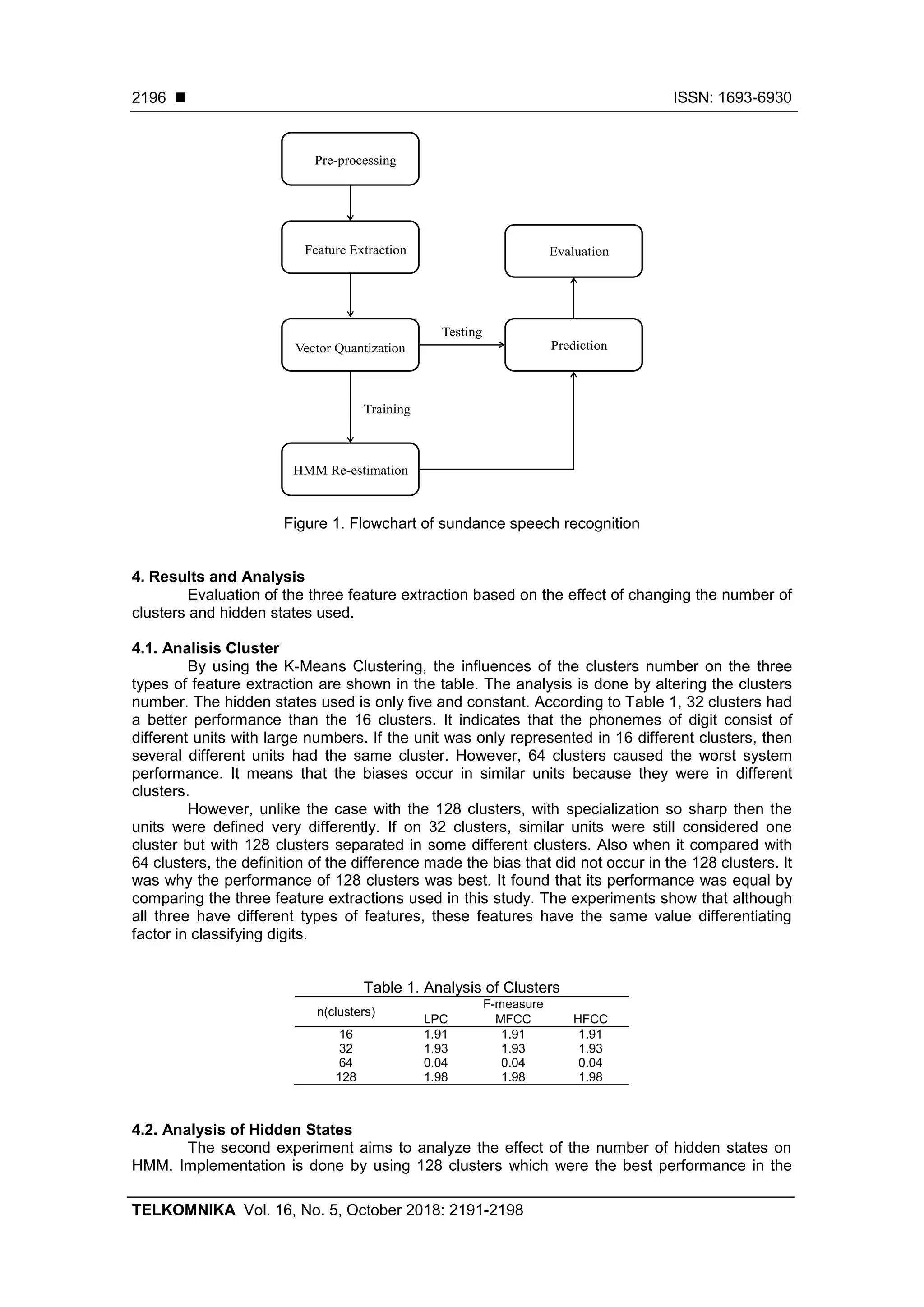
3. System Design
The dataset comes from four different people. The recording is done in the soundproof
room to avoid noise that appears during the process. Every person says the numbers 0 to 9 of
60 times. After that, the data is divided into two parts. 33% of the dataset used
as test data while the rest as training data. The system consists of several stages that are
shown in Figure 1:
a. Pre-processing
Input from the system is wav file. This format is part of the Microsoft RIFF specification
used for storing multimedia files. It starts with the header section and is followed by a chunk
data sequence. Also, it consists of three parts, namely main chunk, chunk format, and chunk
data. The sound signal represented in the discrete form, a series of numbers representing
amplitude in the time domain. In the header file, there is information about the WAV file which
includes the information about of sample rate, and bits per sample, number of channels. Pre-
processing aims to adjust the input system to be processed at later stages. The two primary
processes which occur during pre-processing are centering and normalization.
b. Feature Extraction
It is the process of determining a value or vector that can be used as the object
identifier. Three methods used in this research are Linear Predictive Coding (LPC), Mel
Frequency Cepstral Coefficients (MFCC), and Human Factor Cepstral Coefficient (HFCC)
c. Vector Quantization (VQ)
Vector quantization is the encoding process of the signal vector into some symbols [16].
It consists of two processes. The first process is learning to get the codebook/centroid/cluster
centers. The second is a testing process that transforms data into a symbol feature extraction
results based the obtained codebook. In this study, K-Means Clustering has a role to do this
process.
d. HMM Re-estimation
At this stage, the training data is processed to produce a model that represents the ten
digits by forwarding and backward calculation algorithm.
e. Prediction
All models were evaluated at the HMM re-estimation stage using the test data. A model
that has maximum likelihood become the prediction label.
f. Evaluation
Analysis of the performance of each feature extraction on Sundanese data is evaluated
using F-measure. F-measure is a test parameter based on a combination of precision and
recall [17].

 ISSN: 1693-6930
2196
Figure 1. Flowchart of sundance speech recognition
4. Results and Analysis
Evaluation of the three feature extraction based on the effect of changing the number of
clusters and hidden states used.
4.1. Analisis Cluster
By using the K-Means Clustering, the influences of the clusters number on the three
types of feature extraction are shown in the table. The analysis is done by altering the clusters
number. The hidden states used is only five and constant. According to Table 1, 32 clusters had
a better performance than the 16 clusters. It indicates that the phonemes of digit consist of
different units with large numbers. If the unit was only represented in 16 different clusters, then
several different units had the same cluster. However, 64 clusters caused the worst system
performance. It means that the biases occur in similar units because they were in different
clusters.
However, unlike the case with the 128 clusters, with specialization so sharp then the
units were defined very differently. If on 32 clusters, similar units were still considered one
cluster but with 128 clusters separated in some different clusters. Also when it compared with
64 clusters, the definition of the difference made the bias that did not occur in the 128 clusters. It
was why the performance of 128 clusters was best. It found that its performance was equal by
comparing the three feature extractions used in this study. The experiments show that although
all three have different types of features, these features have the same value differentiating
factor in classifying digits.
Table 1. Analysis of Clusters
n(clusters)
F-measure
LPC MFCC HFCC
16 1.91 1.91 1.91
32 1.93 1.93 1.93
64 0.04 0.04 0.04
128 1.98 1.98 1.98
4.2. Analysis of Hidden States
The second experiment aims to analyze the effect of the number of hidden states on
HMM. Implementation is done by using 128 clusters which were the best performance in the
Pre-processing
Feature Extraction
HMM Re-estimation
Vector Quantization
Training
Testing
Prediction
Evaluation

2197
first experiment. Table 2 shows that the best performance is obtained when the hidden states
are as five, but the worst are nine states. The increase in the number of hidden states has no
trend. With the increasing number of hidden state used, the system more adjusts the correlation
parameters between hidden states. Consequently, there is no significant difference with the
many or few hidden states used. Increasing the number of hidden states did not always cause
the performance of the system. On the other hand, the performance of the three feature
extraction also has the same performance because the value of each feature has a high
similarity.
Table 2. Analysis of Hidden States
n(hidden states)
F-measure
LPC MFCC HFCC
5 1.98 1.98 1.98
6 1.97 1.97 1.97
7 1.98 1.98 1.98
8 1.97 1.97 1.97
9 1.96 1.96 1.96
10 1.97 1.97 1.97
5. Conclusion
Based on Table 1 and 2, it can be concluded that:
a. The performance of the three feature extraction used in this study has the same
performance for Sundanese speech recognition
b. The use of 128 clusters has the best performance so that the distinctive units of the
phoneme can be well separated. Use of too little cluster has a worse performance due to
the different units included in the same cluster. In this study, however, the use of 64
clusters had the worst performance due to bias.
c. There is no trend in changing the number of hidden states. It shows that trials need to be
done to obtain optimal conditions.
For further research, dataset enlargement is required so that the benefits of each feature
extraction can be seen more clearly.
Acknowledgment
This work also supported by Center of Excellence for Higher Education Research Grant
funded by Indonesian Ministry of Research and Higher Education, Contract No.:
718/UN6.3.1/PL/2017.
References
[1] Dario A, et al. Deep speech 2: End-to-end speech recognition in English and mandarin. International
Conference on Machine Learning. 2016: 173-182.
[2] Andrew M, et al. Lexicon-free conversational speech recognition with neural networks. Proceedings
of the 2015 Conference of the North American Chapter of the Association for Computational
Linguistics: Human Language Technologies. 2015: 345-354.
[3] Li D, Dong Y, George E. Deep belief network for large vocabulary continuous speech recognition.
U.S. Patent No 8,972,253, 2015.
[4] Mariko M, Junichi H. Classification of silent speech using support vector machine and relevance
vector machine. Applied Soft Computing. 2014; 20: 95-102.
[5] Nyoman RE, Suyanto, Warih M. Isolated word recognition using ergodic hidden Markov models and
genetic algorithm. Telecommunication Computing Electronics and Control (TELKOMNIKA). 2012;
10(1): 129-136.
[6] Anuja B, et al. Emotion recognition using Speech Processing Using k-nearest neighbor algorithm.
International Journal of Engineering Research and Applications (IJERA). 2014: 2248-9622.
[7] F Jalili, Barani MJ. Speech recognition using combined fuzzy and ant colony algorithm. International
Journal of Electrical and Computer Engineering (IJECE). 2016; 6(5): 2205.
[8] Sukmawati NE, Satriyo A, Sutikno. Comparison of Feature Extraction Mel Frequency Cepstral
Coefficients and Linear Predictive Coding in Automatic Speech Recognition for Indonesian.
Telecommunication Computing Electronics and Control (TELKOMNIKA). 2017; 15(1): 292-298.

 ISSN: 1693-6930
2198
[9] Shivanker DV, Geeta N, Poonam P. Isolated speech recognition using MFCC and DTW. International
Journal of Advanced Research in Electrical, Electronics and Instrumentation Engineering. 2013; 2(8):
4085-4092.
[10] A Benba, A Jilbab, A Hammouch. Using Human Factor Cepstral Coefficient on Multiple Types of
Voice Recordings for Detecting Patients with Parkinson's Disease. IRBM. 2017.
[11] Jun X, et al. Sizing of energy storage and diesel generators in an isolated microgrid using discrete
Fourier transform (DFT). IEEE Transactions on Sustainable Energy. 2014; 5(3): 907-916.
[12] Mark DS, John GH. Exploiting independent filter bandwidth of human factor cepstral coefficients in
automatic speech recognition. The Journal of the Acoustical Society of America. 2004; 116(3): 1774-
1780.
[13] Intan NY, Mohamad IF, Aniati MA. Fuzzy Clustering and Bidirectional Long Short-Term Memory for
Sleep Stages Classification. 2017 International Conference on Soft Computing, Intelligent System
and Information Technology (ICSIIT). Kuta. 2017: 11-16.
[14] Xiao C, Feiping N, Heng H. Multi-View K-Means Clustering on Big Data. IJCAI. 2013: 2598-2604.
[15] Intan NY. The HL, Adiwijaya. Fuzzy hidden Markov models for Indonesian speech classification. J.
Adv. Comput. Intell. Intell. Informatics (JACIII). 2012; 16(3): 381–387.
[16] Intan NY, Mohamad IF, Aniati MA. Bi-directional Long Short-Term Memory using Quantized data of
Deep Belief Networks for Sleep Stage Classification. Procedia Computer Science. Kuta. 2017; 116:
530-538.
[17] Intan NY, Mohamad IF, Aniati MA. Combining deep belief networks and bidirectional long short-term
memory: Case study: Sleep stage classification. 2017 4th International Conference on Electrical
Engineering, Computer Science and Informatics (EECSI). Yogyakarta. 2017: 1-6.

Feature Extraction Analysis for Hidden Markov Models in Sundanese Speech Recognition

More Related Content

What's hot

Similar to Feature Extraction Analysis for Hidden Markov Models in Sundanese Speech Recognition

More from TELKOMNIKA JOURNAL

Recently uploaded

Feature Extraction Analysis for Hidden Markov Models in Sundanese Speech Recognition