This document provides information about online resources available for a data communications and networking textbook. It outlines instructor resources such as PowerPoint slides and a solutions manual, as well as student resources including chapter summaries, quizzes, and glossaries to help learn key concepts from the book. The document encourages both instructors and students to visit the online learning center for these additional educational materials.


![xxii CONTENTS
Chapter 24 Congestion Control and Quality (~j'Service 767
24.1 DATA lRAFFIC 761
Traffic Descriptor 76]
Traffic Profiles 762
24.2 CONGESTION 763
Network Performance 764
24.3 CONGESTION CONTROL 765
Open-Loop Congestion Control 766
Closed-Loop Congestion Control 767
24.4 lWO EXAMPLES 768
Congestion Control in TCP 769
Congestion Control in Frame Relay 773
24.5 QUALITY OF SERVICE 775
Flow Characteristics 775
Flow Classes 776
24.6 TECHNIQUES TO IMPROVE QoS 776
Scheduling 776
Traffic Shaping 777
Resource Reservation 780
Admission Control 780
24.7 INTEGRATED SERVICES 780
Signaling 781
Flow Specification 781
Admission 781
Service Classes 781
RSVP 782
Problems with Integrated Services 784
24.8 DIFFERENTIATED SERVICES 785
DS Field 785
24.9 QoS IN SWITCHED NETWORKS 786
QoS in Frame Relay 787
QoS inATM 789
24.10 RECOMMENDED READING 790
Books 791
24.11 KEY TERMS 791
24.12 SUMMARY 791
24.13 PRACTICE SET 792
Review Questions 792
Exercises 793
PART 6 Application Layer 795
Chapter 25 DO/nain Name Svstem 797
25.1 NAME SPACE 798
Flat Name Space 798
Hierarchical Name Space 798
25.2 DOMAIN NAME SPACE 799
Label 799
Domain Narne 799
Domain 801](https://image.slidesharecdn.com/cnforouzan4e-231013053408-7d177071/85/CN_Forouzan4e-pdf-25-320.jpg)


![xxxii PREFACE
Part Three: Data Link Layer
The third part is devoted to the discussion of the data link layer of the Internet model.
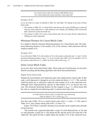
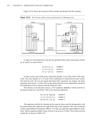
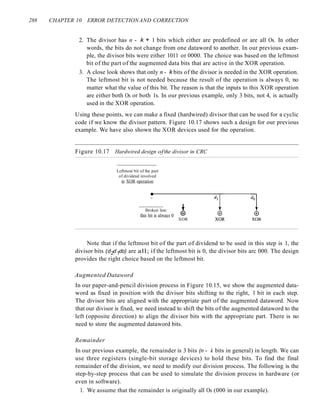
Chapter 10 covers error detection and correction. Chapters 11, 12 discuss issues related
to data link control. Chapters 13 through 16 deal with LANs. Chapters 17 and] 8 are
about WANs. LANs and WANs are examples of networks operating in the first two lay-
ers of the Internet model.
Part Four: Network Layer
The fourth part is devoted to the discussion of the network layer of the Internet model.
Chapter 19 covers IP addresses. Chapters 20 and 21 are devoted to the network layer
protocols such as IP, ARP, ICMP, and IGMP. Chapter 22 discusses delivery, forwarding,
and routing of packets in the Internet.
Part Five: Transport Layer
The fifth part is devoted to the discussion of the transport layer of the Internet model.
Chapter 23 gives an overview of the transport layer and discusses the services and
duties of this layer. It also introduces three transport-layer protocols: UDP, TCP, and
SCTP. Chapter 24 discusses congestion control and quality of service, two issues
related to the transport layer and the previous two layers.
Part Six: Application Layer
The sixth part is devoted to the discussion of the application layer of the Internet model.
Chapter 25 is about DNS, the application program that is used by other application pro-
grams to map application layer addresses to network layer addresses. Chapter 26 to 29
discuss some common applications protocols in the Internet.
Part Seven: Security
The seventh part is a discussion of security. It serves as a prelude to further study in this
subject. Chapter 30 briefly discusses cryptography. Chapter 31 introduces security
aspects. Chapter 32 shows how different security aspects can be applied to three layers
of the Internet model.
Online Learning Center
The McGraw-Hill Online Learning Center contains much additional material. Avail-
able at www.mhhe.com/forouzan. As students read through Data Communications and
Networking, they can go online to take self-grading quizzes. They can also access lec-
ture materials such as PowerPoint slides, and get additional review from animated fig-
ures from the book. Selected solutions are also available over the Web. The solutions to
odd-numbered problems are provided to students, and instructors can use a password to
access the complete set of solutions.
Additionally, McGraw-Hill makes it easy to create a website for your networking
course with an exclusive McGraw-Hill product called PageOut. It requires no prior
knowledge of HTML, no long hours, and no design skills on your part. Instead, Page:-
Out offers a series of templates. Simply fill them with your course information and](https://image.slidesharecdn.com/cnforouzan4e-231013053408-7d177071/85/CN_Forouzan4e-pdf-35-320.jpg)


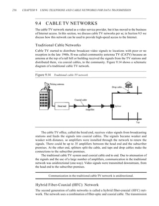
![SECTION 1.5 RECOMMENDED READING 21
electronics manufacturing concerns. Its activities include public awareness education
and lobbying efforts in addition to standards development. In the field of information
technology, the EIA has made significant contributions by defining physical connec-
tion interfaces and electronic signaling specifications for data communication.
Forums
Telecommunications technology development is moving faster than the ability of stan-
dards committees to ratify standards. Standards committees are procedural bodies and
by nature slow-moving. To accommodate the need for working models and agreements
and to facilitate the standardization process, many special-interest groups have devel-
oped forums made up of representatives from interested corporations. The forums
work with universities and users to test, evaluate, and standardize new technologies. By
concentrating their efforts on a particular technology, the forums are able to speed
acceptance and use of those technologies in the telecommunications community. The
forums present their conclusions to the standards bodies.
Regulatory Agencies
All communications technology is subject to regulation by government agencies such
as the Federal Communications Commission (FCC) in the United States. The pur-
pose of these agencies is to protect the public interest by regulating radio, television,
and wire/cable communications. The FCC has authority over interstate and interna-
tional commerce as it relates to communications.
Internet Standards
An Internet standard is a thoroughly tested specification that is useful to and adhered
to by those who work with the Internet. It is a formalized regulation that must be fol-
lowed. There is a strict procedure by which a specification attains Internet standard
status. A specification begins as an Internet draft. An Internet draft is a working docu-
ment (a work in progress) with no official status and a 6-month lifetime. Upon recom-
mendation from the Internet authorities, a draft may be published as a Request for
Comment (RFC). Each RFC is edited, assigned a number, and made available to all
interested parties. RFCs go through maturity levels and are categorized according to
their requirement level.
1.5 RECOMMENDED READING
For more details about subjects discussed in this chapter, we recommend the following
books and sites. The items enclosed in brackets [...] refer to the reference list at the end
of the book.
Books
The introductory materials covered in this chapter can be found in [Sta04] and [PD03].
[Tan03] discusses standardization in Section 1.6.](https://image.slidesharecdn.com/cnforouzan4e-231013053408-7d177071/85/CN_Forouzan4e-pdf-58-320.jpg)


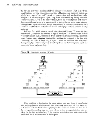


![36 CHAPTER 2 NETWORK MODELS
link layer at B sends a new frame to the data link layer at E. Finally, the data link layer
at E sends a new frame to the data link layer at F. Note that the frames that are
exchanged between the three nodes have different values in the headers. The frame from
A to B has B as the destination address and A as the source address. The frame from B to
E has E as the destination address and B as the source address. The frame from E to F
has F as the destination address and E as the source address. The values of the trailers
can also be different if error checking includes the header of the frame.
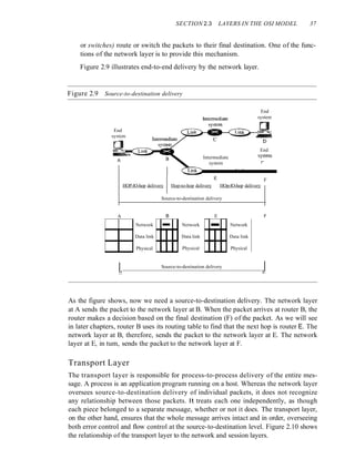
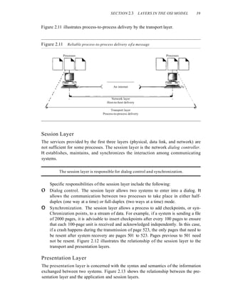
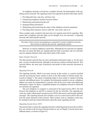
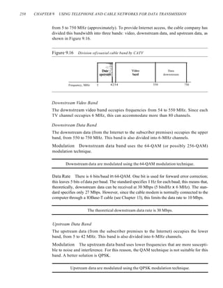
Network Layer
The network layer is responsible for the source-to-destination delivery of a packet,
possibly across multiple networks (links). Whereas the data link layer oversees the
delivery of the packet between two systems on the same network (links), the network
layer ensures that each packet gets from its point of origin to its final destination.
If two systems are connected to the same link, there is usually no need for a net-
work layer. However, if the two systems are attached to different networks (links) with
connecting devices between the networks (links), there is often a need for the network
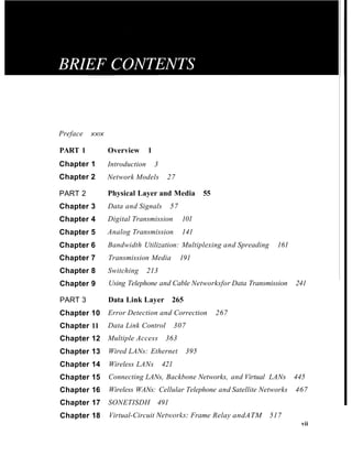
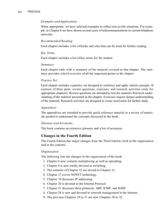
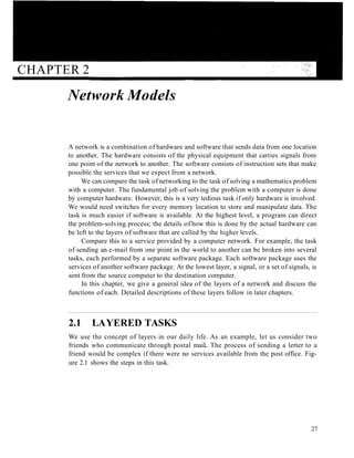
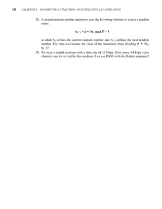
layer to accomplish source-to-destination delivery. Figure 2.8 shows the relationship of
the network layer to the data link and transport layers.
Figure 2.8 Network layer
From transport layer
I
1 -,,-_1
~: Data .1 Packet
I I
To transport layer
...
I
',,- - -H-3- - _]1..
. j
I
. Data,. Packet
i------'-----'-------1
Network
layer
...,
To data link layer
Network
layer
From data link layer
The network layer is responsible for the delivery of individual
packets from the source host to the destination host.
Other responsibilities of the network layer include the following:
o Logical addressing. The physical addressing implemented by the data link layer
handles the addressing problem locally. If a packet passes the network boundary,
we need another addressing system to help distinguish the source and destination
systems. The network layer adds a header to the packet coming from the upper
layer that, among other things, includes the logical addresses of the sender and
receiver. We discuss logical addresses later in this chapter.
o Routing. When independent networks or links are connected to create intemetworks
(network of networks) or a large network, the connecting devices (called routers](https://image.slidesharecdn.com/cnforouzan4e-231013053408-7d177071/85/CN_Forouzan4e-pdf-73-320.jpg)
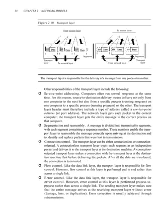


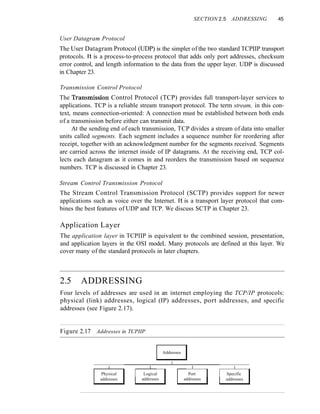
![SECTION 2.4 TCPIIP PROTOCOL SUITE 43
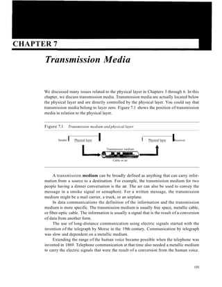
Figure 2.16 TCPIIP and OSI model
IApplication
Applications
J
8GB8GB
I Presentation ... ]
ISession
1
I Transport _ _ _
SC_TP_ _! IL-.-__
TC_P_ _I I UD_P_ _II
I ICMP II IGMP I
Network
IP
(internet)
IRARP II ARP I
IData link
I Physical
Protocols defined by
the underlying networks
(host-to-network)
J
1
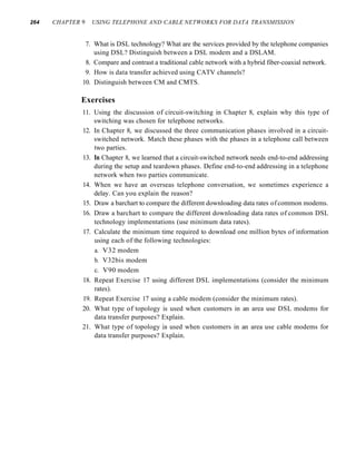
TCP/IP is a hierarchical protocol made up of interactive modules, each of which
provides a specific functionality; however, the modules are not necessarily interdepen-
dent. Whereas the OSI model specifies which functions belong to each of its layers,
the layers of the TCP/IP protocol suite contain relatively independent protocols that
can be mixed and matched depending on the needs of the system. The term hierarchi-
cal means that each upper-level protocol is supported by one or more lower-level
protocols.
At the transport layer, TCP/IP defines three protocols: Transmission Control
Protocol (TCP), User Datagram Protocol (UDP), and Stream Control Transmission
Protocol (SCTP). At the network layer, the main protocol defined by TCP/IP is the
Internetworking Protocol (IP); there are also some other protocols that support data
movement in this layer.
Physical and Data Link Layers
At the physical and data link layers, TCPIIP does not define any specific protocol. It
supports all the standard and proprietary protocols. A network in a TCPIIP internetwork
can be a local-area network or a wide-area network.
Network Layer
At the network layer (or, more accurately, the internetwork layer), TCP/IP supports
the Internetworking Protocol. IP, in turn, uses four supporting protocols: ARP,
RARP, ICMP, and IGMP. Each of these protocols is described in greater detail in later
chapters.](https://image.slidesharecdn.com/cnforouzan4e-231013053408-7d177071/85/CN_Forouzan4e-pdf-80-320.jpg)


![48 CHAPTER 2 NETWORK MODELS
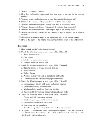
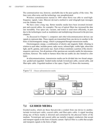
Figure 2.20 IP addresses
AI10
LAN 2
To another
network Y/55
To another XJ44
network
Ph)sical
addl'esscs
changed
LAN 3
-~~_~I~I JRouterll
~tE]
LAN 1
P/95
The computer with logical address A and physical address 10 needs to send a
packet to the computer with logical address P and physical address 95. We use letters to
show the logical addresses and numbers for physical addresses, but note that both are
actually numbers, as we will see later in the chapter.
The sender encapsulates its data in a packet at the network layer and adds two logical
addresses (A and P). Note that in most protocols, the logical source address comes before
the logical destination address (contrary to the order of physical addresses). The network
layer, however, needs to find the physical address of the next hop before the packet can be
delivered. The network layer consults its routing table (see Chapter 22) and finds the
logical address of the next hop (router I) to be F. The ARP discussed previously finds
the physical address of router 1 that corresponds to the logical address of 20. Now the
network layer passes this address to the data link layer, which in tum, encapsulates the
packet with physical destination address 20 and physical source address 10.
The frame is received by every device on LAN 1, but is discarded by all except
router 1, which finds that the destination physical address in the frame matches with its
own physical address. The router decapsulates the packet from the frame to read the log-
ical destination address P. Since the logical destination address does not match the
router's logical address, the router knows that the packet needs to be forwarded. The](https://image.slidesharecdn.com/cnforouzan4e-231013053408-7d177071/85/CN_Forouzan4e-pdf-85-320.jpg)

![50 CHAPTER 2 NETWORK MODELS
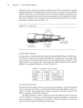
Figure 2.21 Port addresses
a b c
DD
- - - - Data link layer - - --
Internet
j k
DD
The physical addresses change from hop to hop,
but the logical and port addresses usually remain the same.
Example 2.5
As we will see in Chapter 23, a port address is a 16-bit address represented by one decimal num-
her as shown.
753
A 16-bit port address represented as one single number
Specific Addresses
Some applications have user-friendly addresses that are designed for that specific address.
Examples include the e-mail address (for example, forouzan@fhda.edu) and the Universal
Resource Locator (URL) (for example, www.mhhe.com). The first defines the recipient of
an e-mail (see Chapter 26); the second is used to find a document on the World Wide Web
(see Chapter 27). These addresses, however, get changed to the corresponding port and
logical addresses by the sending computer, as we will see in Chapter 25.
2.6 RECOMMENDED READING
For more details about subjects discussed in this chapter, we recommend the following
books and sites. The items enclosed in brackets, [...] refer to the reference list at the
end of the text.](https://image.slidesharecdn.com/cnforouzan4e-231013053408-7d177071/85/CN_Forouzan4e-pdf-87-320.jpg)
![SECTION 2. 7 KEY TERMS 51
Books
Network models are discussed in Section 1.3 of [Tan03], Chapter 2 of [For06], Chapter 2
of [Sta04], Sections 2.2 and 2.3 of [GW04], Section 1.3 of [PD03], and Section 1.7 of
[KR05]. A good discussion about addresses can be found in Section 1.7 of [Ste94].
Sites
The following site is related to topics discussed in this chapter.
o www.osi.org! Information about OS1.
RFCs
The following site lists all RFCs, including those related to IP and port addresses.
o www.ietLorg/rfc.html
2.7 KEY TERMS
access control
Address Resolution Protocol (ARP)
application layer
best-effort delivery
bits
connection control
data link layer
encoding
error
error control
flow control
frame
header
hop-to-hop delivery
host-to-host protocol
interface
Internet Control Message Protocol
(ICMP)
Internet Group Message Protocol (IGMP)
logical addressing
mail service
network layer
node-to-node delivery
open system
Open Systems Interconnection (OSI)
model
peer-to-peer process
physical addressing
physical layer
port address
presentation layer
process-to-process delivery
Reverse Address Resolution Protocol
(RARP)
routing
segmentation
session layer
source-to-destination delivery
Stream Control Transmission Protocol
(SCTP)
synchronization point
TCPIIP protocol suite
trailer
Transmission Control Protocol (TCP)
transmission rate
transport layer
transport level protocols
User Datagram Protocol (UDP)](https://image.slidesharecdn.com/cnforouzan4e-231013053408-7d177071/85/CN_Forouzan4e-pdf-88-320.jpg)


![SECTION 3.2 PERiODIC ANALOG SIGNALS 63
If a signal does not change at all, its frequency is zero.
If a signal changes instantaneously, its frequency is infinite.
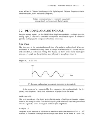
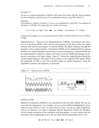
Phase
The term phase describes the position of the waveform relative to time O. If we think of
the wave as something that can be shifted backward or forward along the time axis,
phase describes the amount of that shift. It indicates the status of the first cycle.
Phase describes the position of the waveform relative to time O.
Phase is measured in degrees or radians [360° is 2n rad; 1° is 2n/360 rad, and 1 rad
is 360/(2n)]. A phase shift of 360° corresponds to a shift of a complete period; a phase
shift of 180° corresponds to a shift of one-half of a period; and a phase shift of 90° cor-
responds to a shift of one-quarter of a period (see Figure 3.5).
Figure 3.5 Three sine waves with the same amplitude andfrequency, but different phases
a. 0 degrees
*AAL
1!4TOJ~
b. 90 degrees
c. 180 degrees
•
Time
~
Time
)I
Time
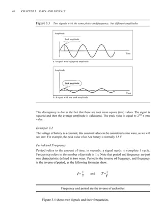
Looking at Figure 3.5, we can say that
I. A sine wave with a phase of 0° starts at time 0 with a zero amplitude. The
amplitude is increasing.
2. A sine wave with a phase of 90° starts at time 0 with a peak amplitude. The
amplitude is decreasing.](https://image.slidesharecdn.com/cnforouzan4e-231013053408-7d177071/85/CN_Forouzan4e-pdf-100-320.jpg)


![70 CHAPTER 3 DATA AND SIGNALS
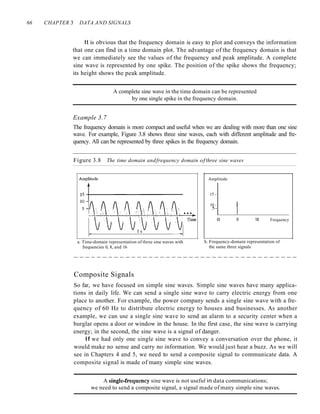
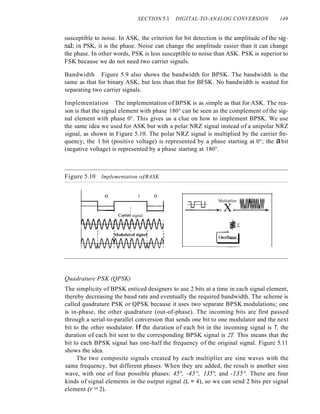
Example 3.10
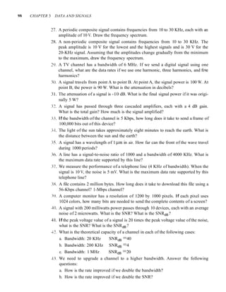
If a periodic signal is decomposed into five sine waves with frequencies of 100, 300, 500, 700,
and 900 Hz, what is its bandwidth? Draw the spectrum, assuming all components have a maxi-
mum amplitude of 10 V.
Solution
Letfh be the highest frequency, fl the lowest frequency, and B the bandwidth. Then
B =fh - it = 900 - 100 =800 Hz
The spectrum has only five spikes, at 100, 300, 500, 700, and 900 Hz (see Figure 3.13).
Figure 3.13 The bandwidthfor Example 3.10
Amplitude
10+-----]
Bandwidth =900 - 100 =800 Hz
100
I,
300 500 700 900
-I
Frequency
Example 3.11
A periodic signal has a bandwidth of 20 Hz. The highest frequency is 60 Hz. What is the lowest
frequency? Draw the spectrum if the signal contains all frequencies of the same amplitude.
Solution
Letfh be the highest frequency,fz the lowest frequency, and B the bandwidth. Then
B =fh - fz :::::} 20 =60 - it =} .ft =60 - 20 =40 Hz
The spectrum contains all integer frequencies. We show this by a series of spikes (see Figure 3.14).
Figure 3.14 The bandwidth for Example 3.11
III
4041 42
I, Bandwidth = 60 - 40 = 20 Hz
585960
·1
Frequency
(Hz)
Example 3.12
A nonperiodic composite signal has a bandwidth of 200 kHz, with a middle frequency of
140 kHz and peak amplitude of 20 V. The two extreme frequencies have an amplitude of 0. Draw
the frequency domain of the signal.](https://image.slidesharecdn.com/cnforouzan4e-231013053408-7d177071/85/CN_Forouzan4e-pdf-107-320.jpg)


![94 CHAPTER 3 DATA AND SIGNALS
Jitter
Another performance issue that is related to delay is jitter. We can roughly say that jitter
is a problem if different packets of data encounter different delays and the application
using the data at the receiver site is time-sensitive (audio and video data, for example).
If the delay for the first packet is 20 ms, for the second is 45 ms, and for the third is
40 ms, then the real-time application that uses the packets endures jitter. We discuss jitter
in greater detail in Chapter 29.
3.7 RECOMMENDED READING
For more details about subjects discussed in this chapter, we recommend the following
books. The items in brackets [...] refer to the reference list at the end of the text.
Books
Data and signals are elegantly discussed in Chapters 1 to 6 of [Pea92]. [CouOl] gives
an excellent coverage about signals in Chapter 2. More advanced materials can be
found in [Ber96]. [Hsu03] gives a good mathematical approach to signaling. Complete
coverage of Fourier Analysis can be found in [Spi74]. Data and signals are discussed in
Chapter 3 of [Sta04] and Section 2.1 of [Tan03].
3.8 KEY TERMS
analog
analog data
analog signal
attenuation
bandpass channel
bandwidth
baseband transmission
bit rate
bits per second (bps)
broadband transmission
composite signal
cycle
decibel (dB)
digital
digital data
digital signal
distortion
Fourier analysis
frequency
frequency-domain
fundamental frequency
harmonic
Hertz (Hz)
jitter
low-pass channel
noise
nonperiodic signal
Nyquist bit rate
peak amplitude
period
periodic signal
phase
processing delay
propagation speed](https://image.slidesharecdn.com/cnforouzan4e-231013053408-7d177071/85/CN_Forouzan4e-pdf-131-320.jpg)


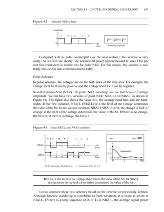
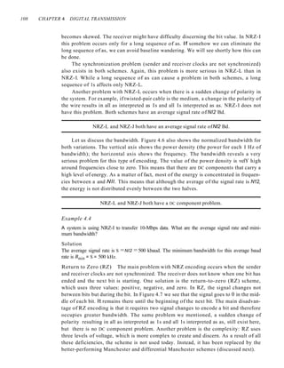


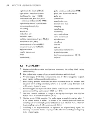
![112 CHAPTER 4 DIGITAL TRANSMISSION
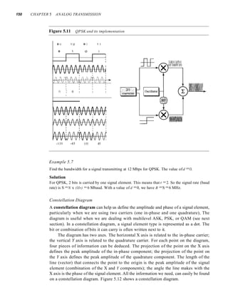
Figure 4.10 Multilevel: 2B1Q scheme
Previous level: Previous level:
positive negative
Next Next Next
bits level level
00 +1 -I
01 +3 -3
10 -I +1
II -3 +3
Transition table
2 fiN
Save =N14
o 1/2
p
1 Bandwidth
0.5
o -
me
00 I II 0] I HI I 0]
I I I
I I
I I
I I
I I
I
Ti
I
I
I
I
I I I
I I I
,
~1
+3
-3
+1
Assuming positive original level
8B6T A very interesting scheme is eight binary, six ternary (8B6T). This code is used
with 100BASE-4T cable, as we will see in Chapter 13. The idea is to encode a pattern of
8 bits as a pattern of 6 signal elements, where the signal has three levels (ternary). In this
type of scheme, we can have 28 =256 different data patterns and 36
=478 different signal
patterns. The mapping table is shown in Appendix D. There are 478 - 256 =222 redundant
signal elements that provide synchronization and error detection. Part of the redundancy is
also used to provide DC balance. Each signal pattern has a weight of 0 or +1 DC values. This
means that there is no pattern with the weight -1. To make the whole stream Dc-balanced,
the sender keeps track of the weight. If two groups of weight 1 are encountered one after
another, the first one is sent as is, while the next one is totally inverted to give a weight of -1.
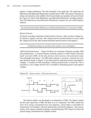
Figure 4.11 shows an example of three data patterns encoded as three signal pat-
terns. The three possible signal levels are represented as -,0, and +. The first 8-bit pat-
tern 00010001 is encoded as the signal pattern -0-0++ with weight 0; the second 8-bit
pattern 01010011 is encoded as - + - + + 0 with weight +1. The third bit pattern should
be encoded as + - - + 0 + with weight +1. To create DC balance, the sender inverts the
actual signal. The receiver can easily recognize that this is an inverted pattern because
the weight is -1. The pattern is inverted before decoding.
Figure 4.11 Multilevel: 8B6T scheme
Time
01()10011
OOOIO()O( O!OIOO()() I
I
Inverted:
pattern :
o+----.--,--..,.....---l---I-+--I--I----L---r--t-----..--r-----It---r----..
+v
-v
-0-0++ -+-++0 +--+0+](https://image.slidesharecdn.com/cnforouzan4e-231013053408-7d177071/85/CN_Forouzan4e-pdf-149-320.jpg)


![SECTION 4.5 KEY TERMS 135
The advantage of synchronous transmission is speed. With no extra bits or gaps to
introduce at the sending end and remove at the receiving end, and, by extension, with
fewer bits to move across the link, synchronous transmission is faster than asynchro-
nous transmission. For this reason, it is more useful for high-speed applications such as
the transmission of data from one computer to another. Byte synchronization is accom-
plished in the data link layer.
We need to emphasize one point here. Although there is no gap between characters
in synchronous serial transmission, there may be uneven gaps between frames.
Isochronous
In real-time audio and video, in which uneven delays between frames are not accept-
able, synchronous transmission fails. For example, TV images are broadcast at the rate
of 30 images per second; they must be viewed at the same rate. If each image is sent
by using one or more frames, there should be no delays between frames. For this type
of application, synchronization between characters is not enough; the entire stream of
bits must be synchronized. The isochronous transmission guarantees that the data
arrive at a fixed rate.
4.4 RECOMMENDED READING
For more details about subjects discussed in this chapter, we recommend the following
books. The items in brackets [...] refer to the reference list at the end of the text.
Books
Digital to digital conversion is discussed in Chapter 7 of [Pea92], Chapter 3 of
[CouOl], and Section 5.1 of [Sta04]. Sampling is discussed in Chapters 15, 16, 17, and
18 of [Pea92], Chapter 3 of [CouO!], and Section 5.3 of [Sta04]. [Hsu03] gives a good
mathematical approach to modulation and sampling. More advanced materials can be
found in [Ber96].
4.5 KEY TERMS
adaptive delta modulation
alternate mark inversion (AMI)
analog-to-digital conversion
asynchronous transmission
baseline
baseline wandering
baud rate
biphase
bipolar
bipolar with 8-zero substitution (B8ZS)
bit rate
block coding
companding and expanding
data element
data rate
DC component
delta modulation (DM)
differential Manchester
digital-to-digital conversion
digitization](https://image.slidesharecdn.com/cnforouzan4e-231013053408-7d177071/85/CN_Forouzan4e-pdf-172-320.jpg)


![156 CHAPTER 5 ANALOG TRANSMISSION
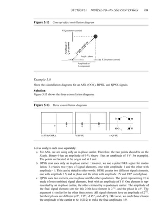
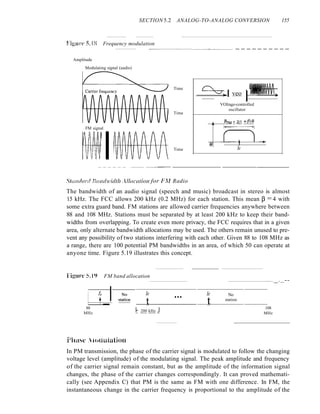
modulating signal; in PM the instantaneous change in the carrier frequency is propor-
tional to the derivative of the amplitude of the modulating signal. Figure 5.20 shows the
relationships of the modulating signal, the carrier signal, and the resultant PM signal.
Figure 5.20 Phase modulation
Amplitude
Modulating signal (audio)
PM signal
Time
Time
Time
VCOI~
I r
~ I
'J 1 dldt
I
1
As Figure 5.20 shows, PM is normally implemented by using a voltage-controlled
oscillator along with a derivative. The frequency of the oscillator changes according to
the derivative of the input voltage which is the amplitude of the modulating signal.
PM Bandwidth
Figure 5.20 also shows the bandwidth of a PM signal. The actual bandwidth is difficult
to determine exactly, but it can be shown empirically that it is several times that of the
analog signal. Although, the formula shows the same bandwidth for FM and PM, the
value of ~ is lower in the case of PM (around 1 for narrowband and 3 for wideband).
The total bandwidth required for PM can be determined from the bandwidth and
maximum amplitude of the modulating signal: BpM = 2(1 + ~ )B.
5.3 RECOMMENDED READING
For more details about subjects discussed in this chapter, we recommend the following
books. The items in brackets [...] refer to the reference list at the end of the text.
Books
Digital-to-analog conversion is discussed in Chapter 14 of [Pea92], Chapter 5 of
[CouOl], and Section 5.2 of [Sta04]. Analog-to-analog conversion is discussed in
Chapters 8 to 13 of [Pea92], Chapter 5 of [CouOl], and Section 5.4 of [Sta04]. [Hsu03]](https://image.slidesharecdn.com/cnforouzan4e-231013053408-7d177071/85/CN_Forouzan4e-pdf-193-320.jpg)
![SECTION 5.5 SUMMARY 157
gives a good mathematical approach to all materials discussed in this chapter. More
advanced materials can be found in [Ber96].
5.4 KEY TERMS
amplitude modulation (AM)
amplitude shift keying (ASK)
analog-to-analog conversion
carrier signal
constellation diagram
digital-to-analog conversion
frequency modulation (PM)
frequency shift keying (FSK)
phase modulation (PM)
phase shift keying (PSK)
quadrature amplitude modulation
(QAM)
5.5 SUMMARY
o Digital-to-analog conversion is the process of changing one of the characteristics
of an analog signal based on the information in the digital data.
o Digital-to-analog conversion can be accomplished in several ways: amplitude shift
keying (ASK), frequency shift keying (FSK), and phase shift keying (PSK).
Quadrature amplitude modulation (QAM) combines ASK and PSK.
o In amplitude shift keying, the amplitude of the carrier signal is varied to create signal
elements. Both frequency and phase remain constant while the amplitude changes.
o In frequency shift keying, the frequency of the carrier signal is varied to represent
data. The frequency of the modulated signal is constant for the duration of one sig-
nal element, but changes for the next signal element if the data element changes.
Both peak amplitude and phase remain constant for all signal elements.
o In phase shift keying, the phase of the carrier is varied to represent two or more dif-
ferent signal elements. Both peak amplitude and frequency remain constant as the
phase changes.
o A constellation diagram shows us the amplitude and phase of a signal element,
particularly when we are using two carriers (one in-phase and one quadrature).
o Quadrature amplitude modulation (QAM) is a combination of ASK and PSK.
QAM uses two carriers, one in-phase and the other quadrature, with different
amplitude levels for each carrier.
o Analog-to-analog conversion is the representation of analog information by an
analog signal. Conversion is needed if the medium is bandpass in nature or if only
a bandpass bandwidth is available to us.
o Analog-to-analog conversion can be accomplished in three ways: amplitude modu-
lation (AM), frequency modulation (FM), and phase modulation (PM).
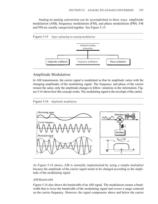
o In AM transmission, the carrier signal is modulated so that its amplitude varies with the
changing amplitudes of the modulating signal. The frequency and phase of the carrier
remain the same; only the amplitude changes to follow variations in the information.
o In PM transmission, the frequency of the carrier signal is modulated to follow the
changing voltage level (amplitude) of the modulating signal. The peak amplitude](https://image.slidesharecdn.com/cnforouzan4e-231013053408-7d177071/85/CN_Forouzan4e-pdf-194-320.jpg)
![158 CHAPTER 5 ANALOG TRANSMISSION
and phase of the carrier signal remain constant, but as the amplitude of the infor-
mation signal changes, the frequency of the carrier changes correspondingly.
o In PM transmission, the phase of the carrier signal is modulated to follow the
changing voltage level (amplitude) of the modulating signal. The peak amplitude
and frequency of the carrier signal remain constant, but as the amplitude of the
information signal changes, the phase of the carrier changes correspondingly.
5.6 PRACTICE SET
Review Questions
1. Define analog transmission.
2. Define carrier signal and its role in analog transmission.
3. Define digital-to-analog conversion.
4. Which characteristics of an analog signal are changed to represent the digital signal
in each of the following digital-to-analog conversion?
a. ASK
b. FSK
c. PSK
d. QAM
5. Which of the four digital-to-analog conversion techniques (ASK, FSK, PSK or
QAM) is the most susceptible to noise? Defend your answer.
6. Define constellation diagram and its role in analog transmission.
7. What are the two components of a signal when the signal is represented on a con- .
stellation diagram? Which component is shown on the horizontal axis? Which is
shown on the vertical axis?
8. Define analog-to-analog conversion?
9. Which characteristics of an analog signal are changed to represent the lowpass analog
signal in each of the following analog-to-analog conversions?
a. AM
b. FM
c. PM
]0. Which of the three analog-to-analog conversion techniques (AM, FM, or PM) is
the most susceptible to noise? Defend your answer.
Exercises
11. Calculate the baud rate for the given bit rate and type of modulation.
a. 2000 bps, FSK
b. 4000 bps, ASK
c. 6000 bps, QPSK
d. 36,000 bps, 64-QAM](https://image.slidesharecdn.com/cnforouzan4e-231013053408-7d177071/85/CN_Forouzan4e-pdf-195-320.jpg)


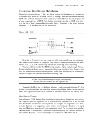

![SECTION 6.1 MULTIPLEXING 171
Example 6.6
Figure 6.14 shows synchronous TOM with a data stream for each input and one data stream for
the output. The unit of data is 1 bit. Find (a) the input bit duration, (b) the output bit duration,
(c) the output bit rate, and (d) the output frame rate.
Figure 6.14 Example 6.6
I Mbps
• •• 1
1 Mbps
• •• 0 0 0 0
1 Mbps
• •• 1 0 0
1 Mbps
• •• 0 0 0
o
o
Frames
••• ffilQI!][Q]QJQliJ1III[Q[QJQli]"
Solution
We can answer the questions as follows:
a. The input bit duration is the inverse of the bit rate: 1/1 Mbps = 1 lls.
b. The output bit duration is one-fourth of the input bit duration, or 1/411s.
c. The output bit rate is the inverse of the output bit duration or 1/4 lls, or 4 Mbps. This can also
be deduced from the fact that the output rate is 4 times as fast as any input rate; so the output
rate =4 x 1 Mbps =4 Mbps.
d. The frame rate is always the same as any input rate. So the frame rate is 1,000,000 frames per
second. Because we are sending 4 bits in each frame, we can verify the result of the previous
question by multiplying the frame rate by the number of bits per frame.
Example 6.7
Four l-kbps connections are multiplexed together. A unit is I bit. Find (a) the duration of I bit
before multiplexing, (b) the transmission rate of the link, (c) the duration of a time slot, and
(d) the duration of a frame.
Solution
We can answer the questions as follows:
a. The duration of 1 bit before multiplexing is 1/1 kbps, or 0.001 s (l ms).
b. The rate of the link is 4 times the rate of a connection, or 4 kbps.
c. The duration of each time slot is one-fourth of the duration of each bit before multiplexing,
or 1/4 ms or 250 I.ls. Note that we can also calculate this from the data rate of the link, 4 kbps.
The bit duration is the inverse of the data rate, or 1/4 kbps or 250 I.ls.
d. The duration of a frame is always the same as the duration of a unit before multiplexing, or
I ms. We can also calculate this in another way. Each frame in this case has fouf time slots.
So the duration of a frame is 4 times 250 I.ls, or I ms.
Interleaving
TDM can be visualized as two fast-rotating switches, one on the multiplexing side and
the other on the demultiplexing side. The switches are synchronized and rotate at the
same speed, but in opposite directions. On the multiplexing side, as the switch opens](https://image.slidesharecdn.com/cnforouzan4e-231013053408-7d177071/85/CN_Forouzan4e-pdf-208-320.jpg)


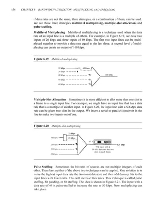


![SECTION 6.4 KEY TERMS 185
Figure 6.33 DSSS example
Original 1-- _
signal
Spreading 1---+--+--1-+--1---
code
Spread f----t-+-+-i--+---
signal
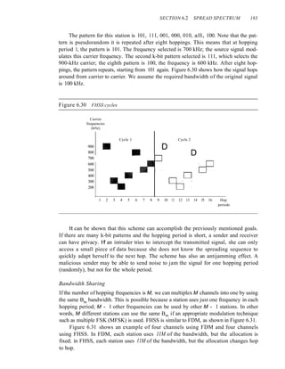
Bandwidth Sharing
Can we share a bandwidth in DSSS as we did in FHSS? The answer is no and yes. If we
use a spreading code that spreads signals (from different stations) that cannot be combined
and separated, we cannot share a bandwidth. For example, as we will see in Chapter 14,
some wireless LANs use DSSS and the spread bandwidth cannot be shared. However, if
we use a special type of sequence code that allows the combining and separating of spread
signals, we can share the bandwidth. As we will see in Chapter 16, a special spreading code
allows us to use DSSS in cellular telephony and share a bandwidth between several users.
6.3 RECOMMENDED READING
For more details about subjects discussed in this chapter, we recommend the following
books. The items in brackets [...] refer to the reference list at the end of the text.
Books , '-
Multiplexing is elegantly discussed in Chapters 19 of [Pea92]. [CouOI] gives excellent
coverage of TDM and FDM in Sections 3.9 to 3.11. More advanced materials can be
found in [Ber96]. Multiplexing is discussed in Chapter 8 of [Sta04]. A good coverage of
spread spectrum can be found in Section 5.13 of [CouOl] and Chapter 9 of [Sta04].
6.4 KEY TERMS
analog hierarchy
Barker sequence
channel
chip
demultiplexer (DEMUX)
dense WDM (DWDM)
digital signal (DS) service
direct sequence spread spectrum (DSSS)
Eline
framing bit
frequency hopping spread spectrum
(FSSS)](https://image.slidesharecdn.com/cnforouzan4e-231013053408-7d177071/85/CN_Forouzan4e-pdf-222-320.jpg)


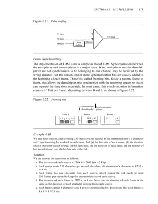
![SECTION 7.1 GUIDED MEDIA 195
Figure 7.5 UTP connector
nrnln
12345678
RJ-45 Male
Figure 7.6 UTP performance
18 gauge
26 gauge
Gauge Diameter (inches)
18 0.0403
22 0.02320
24 0.02010
26 0.0159
18
2 E::::::::..------
4
20
16
]' 14
iIi
::3- 12
<::
.g
'" 10
:I
<::
"
~ 8
6
10 100 1000
!(kHz)
Applications
Twisted-pair cables are used in telephone lines to provide voice and data channels. The
local loop-the line that connects subscribers to the central telephone office---commonly
consists of unshielded twisted-pair cables. We discuss telephone networks in Chapter 9.
The DSL lines that are used by the telephone companies to provide high-data-rate
connections also use the high-bandwidth capability of unshielded twisted-pair cables.
We discuss DSL technology in Chapter 9.
Local-area networks, such as lOBase-T and lOOBase-T, also use twisted-pair cables.
We discuss these networks in Chapter 13.
Coaxial Cable
Coaxial cable (or coax) carries signals of higher frequency ranges than those in twisted-
pair cable, in part because the two media are constructed quite differently. Instead of](https://image.slidesharecdn.com/cnforouzan4e-231013053408-7d177071/85/CN_Forouzan4e-pdf-232-320.jpg)


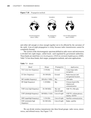


![208 CHAPTER 7 TRANSMISSION MEDIA
Applications
The infrared band, almost 400 THz, has an excellent potential for data transmission.
Such a wide bandwidth can be used to transmit digital data with a very high data rate.
The Infrared Data Association (IrDA), an association for sponsoring the use of infrared
waves, has established standards for using these signals for communication between
devices such as keyboards, mice, PCs, and printers. For example, some manufacturers
provide a special port called the IrDA port that allows a wireless keyboard to commu-
nicate with a PC. The standard originally defined a data rate of 75 kbps for a distance
up to 8 m. The recent standard defines a data rate of 4 Mbps.
Infrared signals defined by IrDA transmit through line of sight; the IrDA port on
the keyboard needs to point to the PC for transmission to occur.
Infrared signals can be used for short-range communication
in a closed area using line-of-sight propagation.
7.3 RECOMMENDED READING
For more details about subjects discussed in this chapter, we recommend the following
books. The items in brackets [...] refer to the reference list at the end of the text.
Books
Transmission media is discussed in Section 3.8 of [GW04], Chapter 4 of [Sta04], Sec-
tion 2.2 and 2.3 of [Tan03]. [SSS05] gives a full coverage of transmission media.
7.4 KEY TERMS
angle of incidence
Bayone-Neil-Concelman (BNC)
connector
cladding
coaxial cable
core
critical angle
electromagnetic spectrum
fiber-optic cable
gauge
ground propagation
guided media
horn antenna
infrared wave
IrDA port
line-of-sight propagation
microwave
MT-RJ
multimode graded-index fiber
multimode step-index fiber
omnidirectional antenna
optical fiber
parabolic dish antenna
Radio Government (RG) number
radio wave
reflection
refraction
RJ45](https://image.slidesharecdn.com/cnforouzan4e-231013053408-7d177071/85/CN_Forouzan4e-pdf-245-320.jpg)

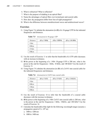


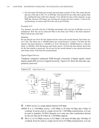
![224 CHAPTER 8 SWITCHING
Figure 8.12 Switch and tables in a virtual-circuit network
Incoming Outgoing
Port VCl Port VCl
1 14 3 22
1 77 2 41
~'~
I Data ~I Data [EJ-+
lA3 I Data @]-+
2
~t
Figure 8.13 Source-to-destination data transfer in a virtual-circuit network
Incoming Outgoing
Port VCl Port VCl
I 14 3 66
Incoming Outgoing
Port VCl Port VCI
2 22 3 77
Incoming Outgoing
Port VCI Port VCl
1 66 2 22
Setup Request A setup request frame is sent from the source to the destination.
Figure 8.14 shows the process.
a. Source A sends a setup frame to switch 1.
b. Switch 1 receives the setup request frame. It knows that a frame going from A to B
goes out through port 3. How the switch has obtained this information is a point
covered in future chapters. The switch, in the setup phase, acts as a packet switch;
it has a routing table which is different from the switching table. For the moment,
assume that it knows the output port. The switch creates an entry in its table for](https://image.slidesharecdn.com/cnforouzan4e-231013053408-7d177071/85/CN_Forouzan4e-pdf-261-320.jpg)

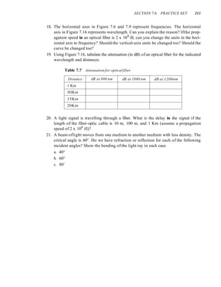
![SECTION 8.4 STRUCTURE OF A SWITCH 227
Figure 8.16 Delay in a virtual-circuit network
I ~I
"
~ [--~---------------
~ ,
~
]
1;'ransmission
tIme
Time Time Time Time
and a teardown delay (which includes transmission and propagation in one direction).
We ignore the processing time in each switch. The total delay time is
Total delay = 3T + 3't + setup delay + teardown delay
Circuit-Switched Technology in WANs
As we will see in Chapter 18, virtual-circuit networks are used in switched WANs such
as Frame Relay and ATM networks. The data link layer of these technologies is well
suited to the virtual-circuit technology.
Switching at the data link layer in a switched WAN is normally
implemented by using virtual-circuit techniques.
8.4 STRUCTURE OF A SWITCH
We use switches in circuit-switched and packet-switched networks. In this section, we
discuss the structures of the switches used in each type of network.
Structure of Circuit Switches
Circuit switching today can use either of two technologies: the space-division switch or
the time-division switch.
Space-Division Switch
In space-division switching, the paths in the circuit are separated from one another
spatially. This technology was originally designed for use in analog networks but is
used currently in both analog and digital networks. It has evolved through a long history
of many designs.](https://image.slidesharecdn.com/cnforouzan4e-231013053408-7d177071/85/CN_Forouzan4e-pdf-264-320.jpg)

![230 CHAPTER 8 SWITCHING
Clos investigated the condition of nonblocking in multistage switches and came up
with the following formula. In a nonblocking switch, the number of middle-stage
switches must be at least 2n - 1. In other words, we need to have k 2 2n - 1.
Note that the number of crosspoints is still smaller than that in a single-stage
switch. Now we need to minimize the number of crosspoints with a fixed N by using
the Clos criteria. We can take the derivative of the equation with respect to n (the only
variable) and find the value of n that makes the result zero. This n must be equal to or
greater than (N/2)1/2. In this case, the total number of crosspoints is greater than or equal
to 4N [(2N) 112 -1]. In other words, the minimum number of crosspoints according to the
Clos criteria is proportional to N3/2.
According to Clos criterion:
n =(NI2)1/2
k>2n-1
Total number of crosspoints 2 4N [(2N)1/2 -1]
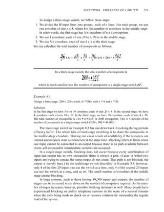
Example 8.4
Redesign the previous three-stage, 200 x 200 switch, using the Clos criteria with a minimum
number of crosspoints.
Solution
We let n = (200/2)1/2, or n = 10. We calculate k = 2n - 1= 19. In the first stage, we have 200/10,
or 20, crossbars, each with lOX 19 crosspoints. In the second stage, we have 19 crossbars,
each with 10 X 10 crosspoints. In the third stage, we have 20 crossbars each with 19 X 10
crosspoints. The total number of crosspoints is 20(10 X 19) + 19(10 X 10) + 20(19 XlO) =
9500. If we use a single-stage switch, we need 200 X 200 =40,000 crosspoints. The number
of crosspoints in this three-stage switch is 24 percent that of a single-stage switch. More
points are needed than in Example 8.3 (5 percent). The extra crosspoints are needed to prevent
blocking.
A multistage switch that uses the Clos criteria and a minimum number of crosspoints
still requires a huge number of crosspoints. For example, to have a 100,000 input/output
switch, we need something close to 200 million crosspoints (instead of 10 billion). This
means that if a telephone company needs to provide a switch to connect 100,000 tele-
phones in a city, it needs 200 million crosspoints. The number can be reduced if we
accept blocking. Today, telephone companies use time-division switching or a combina-
tion of space- and time-division switches, as we will see shortly.
Time-Division Switch
Time-division switching uses time-division multiplexing (TDM) inside a switch. The
most popular technology is called the time-slot interchange (TSI).
Time-Slot Interchange Figure 8.19 shows a system connecting four input lines to
four output lines. Imagine that each input line wants to send data to an output line
according to the following pattern:](https://image.slidesharecdn.com/cnforouzan4e-231013053408-7d177071/85/CN_Forouzan4e-pdf-267-320.jpg)


![SECTION 8.6 KEY TERMS 235
Figure 8.26 Batcher-banyan switch
Banyan switch
O~
l~
6~
7~
Batcher
switch
Trap
module
~2
~3
~--+ro ~"'lr-r ~ 4
~5
~6
~7
Batcher-Banyan Switch The problem with the banyan switch is the possibility of
internal collision even when two packets are not heading for the same output port. We
can solve this problem by sorting the arriving packets based on their destination port.
K. E. Batcher designed a switch that comes before the banyan switch and sorts the
incoming packets according to their final destinations. The combination is called the
Batcher-banyan switch. The sorting switch uses hardware merging techniques, but we
do not discuss the details here. Normally, another hardware module called a trap is
added between the Batcher switch and the banyan switch (see Figure 8.26) The trap
module prevents duplicate packets (packets with the same output destination) from
passing to the banyan switch simultaneously. Only one packet for each destination is
allowed at each tick; if there is more than one, they wait for the next tick.
8.5 RECOMMENDED READING
For more details about subjects discussed in this chapter, we recommend the following
books. The items in brackets [...] refer to the reference list at the end of the text.
Books
Switching is discussed in Chapter 10 of [Sta04] and Chapters 4 and 7 of [GW04]. Circuit-
switching is fully discussed in [BELOO].
8.6 KEY TERMS
banyan switch
Batcher-banyan switch
blocking
circuit switching
circuit-switched network
crossbar switch
crosspoint
data transfer phase
datagram
datagram network
end system
input port](https://image.slidesharecdn.com/cnforouzan4e-231013053408-7d177071/85/CN_Forouzan4e-pdf-272-320.jpg)
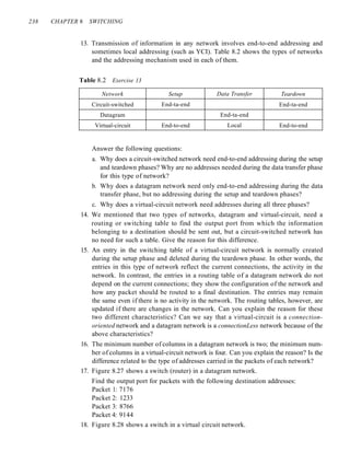
![SECTION 8.8 PRACTICE SET 239
Figure 8.27 Exercise 17
Destination Output
address port
1233 3
1456 2
3255 1
4470 4
7176 2
8766 3
9144 2
4
2 3
Figure 8.28 Exercise 18
Incoming Outgoing
Port VCI Port VCI
1 14 3 22
2 71 4 41
2 92 1 45
3 58 2 43
3 78 2 70
4 56 3 11
2
4
Find the output port and the output VCI for packets with the following input port
and input VCI addresses:
Packet 1: 3, 78
Packet 2: 2, 92
Packet 3: 4, 56
Packet 4: 2, 71
19. Answer the following questions:
a. Can a routing table in a datagram network have two entries with the same destina-
tion address? Explain.
b. Can a switching table in a virtual-circuit network have two entries with the same
input port number? With the same output port number? With the same incoming
VCls? With the same outgoing VCls? With the same incoming values (port, VCI)?
With the same outgoing values (port, VCI)?
20. It is obvious that a router or a switch needs to do searching to find information in
the corresponding table. The searching in a routing table for a datagram network is
based on the destination address; the searching in a switching table in a virtual-
circuit network is based on the combination of incoming port and incoming VCI.
Explain the reason and define how these tables must be ordered (sorted) based on
these values.
2]. Consider an n X k crossbar switch with n inputs and k outputs.
a. Can we say that switch acts as a multiplexer if n > k?
b. Can we say that switch acts as a demultiplexer if n < k?](https://image.slidesharecdn.com/cnforouzan4e-231013053408-7d177071/85/CN_Forouzan4e-pdf-276-320.jpg)


![SECTION 9. 7 KEY TERMS 261
CMs and CMTSs for the minislots used for timesharing of the upstream channels.
We will learn about this timesharing when we discuss contention protocols in
Chapter 12.
4. The CM sends a packet to the ISP, asking for the Internet address.
5. The CM and CMTS then exchange some packets to establish security parameters,
which are needed for a public network such as cable TV.
6. The CM sends its unique identifier to the CMTS.
7. Upstream communication can start in the allocated upstream channel; the CM can
contend for the minislots to send data.
Downstream Communication
In the downstream direction, the communication is much simpler. There is no conten-
tion because there is only one sender. The CMTS sends the packet with the address of
the receiving eM, using the allocated downstream channel.
9.6 RECOMMENDED READING
For more details about subjects discussed in this chapter, we recommend the following
books. The items in brackets [...] refer to the reference list at the end of the text.
Books
[CouOl] gives an interesting discussion about telephone systems, DSL technology,
and CATV in Chapter 8. [Tan03] discusses telephone systems and DSL technology in
Section 2.5 and CATV in Section 2.7. [GW04] discusses telephone systems in Sec-
tion 1.1.1 and standard modems in Section 3.7.3. A complete coverage of residential
broadband (DSL and CATV) can be found in [Max99].
9.7 KEY TERMS
56Kmodem
800 service
900 service
ADSL Lite
ADSLmodem
analog leased service
analog switched service
asymmetric DSL (ADSL)
cable modem (CM)
cable modem transmission system
(CMTS)
cable TV network
common carrier
community antenna TV (CATV)
competitive local exchange carrier
(CLEC)
Data Over Cable System Interface
Specification (DOCSIS)
demodulator
digital data service (DDS)
digital service
digital subscriber line (DSL)
digital subscriber line access multiplexer
(DSLAM)
discrete multitone technique (DMT)
distribution hub](https://image.slidesharecdn.com/cnforouzan4e-231013053408-7d177071/85/CN_Forouzan4e-pdf-298-320.jpg)


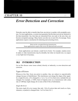


![SECTION 10.4 CYCLIC CODES 287
Decoder
The codeword can change during transmission. The decoder does the same division
process as the encoder. The remainder of the division is the syndrome. If the syndrome
is all Os, there is no error; the dataword is separated from the received codeword and
accepted. Otherwise, everything is discarded. Figure 10.16 shows two cases: The left-
hand figure shows the value of syndrome when no error has occurred; the syndrome is
000. The right-hand part of the figure shows the case in which there is one single error.
The syndrome is not all Os (it is OIl).
Figure 10.16 Division in the CRC decoderfor two cases
Codeword 11 o 0 011 1 0 I
Division t
I 0 I 0
1 0 1 1) 1 0 0 o 1 1 o _Codeword
1 0 1
1+1
0 I I 1
0 0 o ()
1 I
0 1
o 0 0
011
~Syndrome
t
Dataword_
discarded
Divisor
You may be wondering how the divisor] 011 is chosen. Later in the chapter we present
some criteria, but in general it involves abstract algebra.
Hardware Implementation
One of the advantages of a cyclic code is that the encoder and decoder can easily and
cheaply be implemented in hardware by using a handful of electronic devices. Also, a
hardware implementation increases the rate of check bit and syndrome bit calculation.
In this section, we try to show, step by step, the process. The section, however, is
optional and does not affect the understanding of the rest of the chapter.
Divisor
Let us first consider the divisor. We need to note the following points:
1. The divisor is repeatedly XORed with part of the dividend.](https://image.slidesharecdn.com/cnforouzan4e-231013053408-7d177071/85/CN_Forouzan4e-pdf-324-320.jpg)
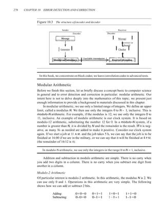
![SECTION 10.4 CYCLIC CODES 289
2. At each time click (arrival of 1 bit from an augmented dataword), we repeat the
following two actions:
a. We use the leftmost bit to make a decision about the divisor (011 or 000).
b. The other 2 bits of the remainder and the next bit from the augmented dataword
(total of 3 bits) are XORed with the 3-bit divisor to create the next remainder.
Figure 10.18 shows this simulator, but note that this is not the final design; there will be
more improvements.
Figure 10.18 Simulation ofdivision in CRC encoder
.C; /~~~ /~I~ o~ Augmented dataword
,-(B~ I 0 0 0 0 0
TIme: I .iLk' ,
, , ,
Time:2L:1i
,
t -' ,~l~o
ot~
/-@ 0 /~@~ 0 0 00
,o?:-'mMft ,
/ , ,
Time: 3 L:i!&
,
°t ' ,~1~0
°t--dJ
/-(B 1 /-@~ 0 00
'p' ~~~
,
/ , ,
Time:4L:1i
,
/~I~ ,~1~1
ot~
/-(B 0 0 0 0
8~:<8?::<8ffi) ,
/
, ,
Time: 5 L::Ii /~~--dJ
t '
,~l~o
/~l±)~ 0 0
,
/ , ,
Time:6~
. It -'
,!1~0
ot~
/ -l±) 0 /-l±)~ 0
,
/ , ,
Time:7l1' °t--dJ °t ' ol
/-0 1 ,'-0~ ,-(B~o
~- /
/ / ,
/ / /
II oJ IT]
~. ''"'-<
I
Final remainder
At each clock tick, shown as different times, one of the bits from the augmented
dataword is used in the XOR process. If we look carefully at the design, we have seven
steps here, while in the paper-and-pencil method we had only four steps. The first three
steps have been added here to make each step equal and to make the design for each step
the same. Steps 1, 2, and 3 push the first 3 bits to the remainder registers; steps 4, 5, 6,
and 7 match the paper-and-pencil design. Note that the values in the remainder register
in steps 4 to 7 exactly match the values in the paper-and-pencil design. The final remain-
der is also the same.
The above design is for demonstration purposes only. It needs simplification to be
practical. First, we do not need to keep the intermediate values of the remainder bits;
we need only the final bits. We therefore need only 3 registers instead of 24. After the
XOR operations, we do not need the bit values of the previous remainder. Also, we do](https://image.slidesharecdn.com/cnforouzan4e-231013053408-7d177071/85/CN_Forouzan4e-pdf-326-320.jpg)


![SECTION fO.7 KEY TERMS 301
leftmost dight (3) as the carry in the second column. The process is repeated for each column.
Hexadecimal numbers are reviewed in Appendix B.
Note that if there is any corruption, the checksum recalculated by the receiver is not all as.
We leave this an exercise.
Performance
The traditional checksum uses a small number of bits (16) to detect errors in a message
of any size (sometimes thousands of bits). However, it is not as strong as the CRC in
error-checking capability. For example, if the value of one word is incremented and the
value of another word is decremented by the same amount, the two errors cannot be
detected because the sum and checksum remain the same. Also if the values of several
words are incremented but the total change is a multiple of 65535, the sum and the
checksum does not change, which means the errors are not detected. Fletcher and Adler
have proposed some weighted checksums, in which each word is multiplied by a num-
ber (its weight) that is related to its position in the text. This will eliminate the first
problem we mentioned. However, the tendency in the Internet, particularly in designing
new protocols, is to replace the checksum with a CRC.
10.6 RECOMMENDED READING
For more details about subjects discussed in this chapter, we recommend the following
books. The items in brackets [...] refer to the reference list at the end of the text.
Books
Several excellent book are devoted to error coding. Among them we recommend [Ham80],
[Zar02], [Ror96], and [SWE04].
RFCs
A discussion of the use of the checksum in the Internet can be found in RFC 1141.
10.7 KEY TERMS
block code
burst error
check bit
checksum
codeword
convolution code
cyclic code
cyclic redundancy check (CRC)
dataword
error
error correction
error detection
forward error correction
generator polynomial
Hamming code
Hamming distance
interference
linear block code
minimum Hamming distance
modular arithmetic](https://image.slidesharecdn.com/cnforouzan4e-231013053408-7d177071/85/CN_Forouzan4e-pdf-338-320.jpg)


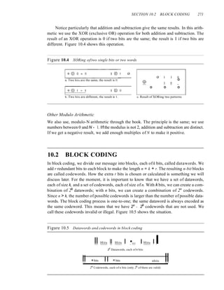
![SECTION 11.4 NOISELESS CHANNELS 313
sender to receiver. We assume that the receiver can immediately handle any frame it
receives with a processing time that is small enough to be negligible. The data link
layer ofthe receiver immediately removes the header from the frame and hands the data
packet to its network layer, which can also accept the packet immediately. In other
words, the receiver can never be overwhelmed with incoming frames.
Design
There is no need for flow control in this scheme. The data link layer at the sender site
gets data from its network layer, makes a frame out of the data, and sends it. The data
link layer at the receiver site receives a frame from its physical layer, extracts data from
the frame, and delivers the data to its network layer. The data link layers of the sender
and receiver provide transmission services for their network layers. The data link layers
use the services provided by their physical layers (such as signaling, multiplexing, and
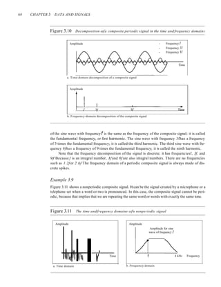
so on) for the physical transmission of bits. Figure 11.6 shows a design.
Figure 11.6 The design ofthe simplest protocol with no flow or error control
Sender Receiver
Network
Data link
Physical
Get data Delivrdata
t I
I ...
t I
Send frame Receive frame
Data frames -+-
I ~~~~~~~ I
Network
Data link
Physical
Repeat forever
Event: ){otifu:ationfrom
physlclU iaye]"
We need to elaborate on the procedure used by both data link layers. The sender site
cannot send a frame until its network layer has a data packet to send. The receiver site
cannot deliver a data packet to its network layer until a frame arrives. If the protocol is
implemented as a procedure, we need to introduce the idea of events in the protocol. The
procedure at the sender site is constantly running; there is no action until there is a request
from the network layer. The procedure at the receiver site is also constantly rulming, but
there is no action until notification from the physical layer arrives. Both procedures are
constantly running because they do not know when the corresponding events will occur.](https://image.slidesharecdn.com/cnforouzan4e-231013053408-7d177071/85/CN_Forouzan4e-pdf-350-320.jpg)

![SECTION 1I.4 NOISELESS CHANNELS 317
acknowledged. We know that two arrival events cannot happen one after another because the
channel is error-free and does not duplicate the frames. The requests from the network layer,
however, may happen one after another without an arrival event in between. We need somehow to
prevent the immediate sending of the data frame. Although there are several methods, we have
used a simple canSend variable that can either be true or false. When a frame is sent, the variable
is set to false to indicate that a new network request cannot be sent until canSend is true. When an
ACK is received, canSend is set to true to allow the sending of the next frame.
Algorithm 11.4 shows the procedure at the receiver site.
Algorithm 11.4 Receiver-site algorithm for Stop-and-Wait Protocol
WaitForEvent(); II Sleep until an event occurf
if(Event(ArrivalNotification)} IIData frame arrives
{
/IDeliver data to network layex
IISend an ACK frame
IIRepeat forever
ReceiveFrame(};
ExtractData(}i
Deliver(data};
SendFrame();
}
1 while (true)
2 {
3
4
5
6
7
8
9
10
11 }
Analysis This is very similar to Algorithm 11.2 with one exception. After the data frame
arrives, the receiver sends an ACK frame (line 9) to acknowledge the receipt and allow the sender
to send the next frame.
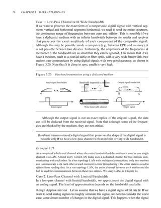
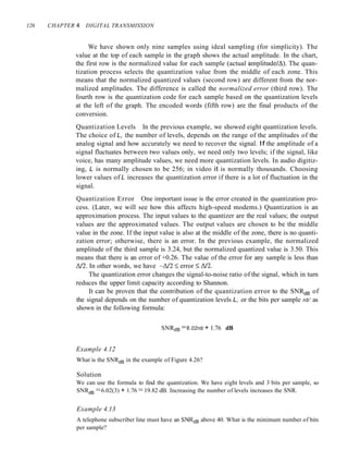
Example 11.2
Figure 11.9 shows an example of communication using this protocol. It is still very simple. The
sender sends one frame and waits for feedback from the receiver. When the ACK arrives, the
sender sends the next frame. Note that sending two frames in the protocol involves the sender in
four events and the receiver in two events.
Figure 11.9 Flow diagramfor Example 1I.2
Sender
INA]
Receiver
rIJ
Arrival
Frame
Arrival :
I
Request
ReqUest~~
:
I Arrival
I
1 . AC'i..
Arrival' I
• 1
t t
Time Time](https://image.slidesharecdn.com/cnforouzan4e-231013053408-7d177071/85/CN_Forouzan4e-pdf-354-320.jpg)


![SECTION 11.5 NOISY CHANNELS 323
Figure 11.11 Flow diagram for Example 11.3
Sender Receiver
Rn
~9_ET9Ihql!J Arrival
Rn
:~~[nQIrIqUJ Arrival
Rn
~o:-(:-o+o~-(: Arrival
1 __1__ :_J...!.1_!.._.!
Discard, duplicate
m
I
I
I
ACK 1]
---------11
1
t
Time
5n
Request f9"1iJ-9J]~3iff~
Sn
Request @rU9I(~qn~
5n
Time-out f9"rtr9n_:_qff~
Stop
Start cp
Stop l
Stop
Start It
5"
Time-out It Time-out :-6~i+f~0i "1-'
restart ,__!._l£J__'__1__1
Time-out
restart
The system can send 20,000 bits during the time it takes for the data to go from the sender to the
receiver and then back again. However, the system sends only 1000 bits. We can say that the link
utilization is only 1000/20,000, or 5 percent. For this reason, for a link with a high bandwidth or
long delay, the use of Stop-and-Wait ARQ wastes the capacity of the link.
Example 11.5
What is the utilization percentage of the link in Example 11.4 if we have a protocol that can send
up to 15 frames before stopping and worrying about the acknowledgments?
Solution
The bandwidth-delay product is still 20,000 bits. The system can send up to 15 frames or
15,000 bits during a round trip. This means the utilization is 15,000/20,000, or 75 percent. Of
course, if there are damaged frames, the utilization percentage is much less because frames
have to be resent.
Pipelining
In networking and in other areas, a task is often begun before the previous task has ended.
This is known as pipelining. There is no pipelining in Stop-and-Wait ARQ because we
need to wait for a frame to reach the destination and be acknowledged before the next
frame can be sent. However, pipelining does apply to our next two protocols because](https://image.slidesharecdn.com/cnforouzan4e-231013053408-7d177071/85/CN_Forouzan4e-pdf-360-320.jpg)


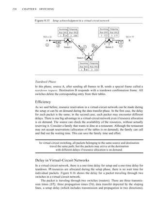
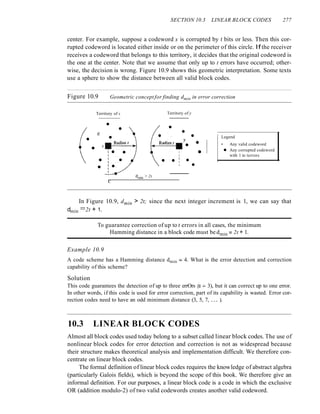
![SECTION 11.5 NOISY CHANNELS 333
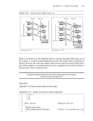
Windows
The Selective Repeat Protocol also uses two windows: a send window and a receive win-
dow. However, there are differences between the windows in this protocol and the ones in
Go-Back-N. First, the size of the send window is much smaller; it is 2m
-
I
. The reason for
this will be discussed later. Second, the receive window is the same size as the send window.
The send window maximum size can be 2m- I
. For example, if m = 4, the
sequence numbers go from 0 to 15, but the size of the window is just 8 (it is 15 in
the Go-Back-N Protocol). The smaller window size means less efficiency in filling the
pipe, but the fact that there are fewer duplicate frames can compensate for this.
The protocol uses the same variables as we discussed for Go-Back-N. We show the
Selective Repeat send window in Figure 11.18 to emphasize the size. Compare it with
Figure 11.12.
Figure 11.18 Send window for Selective Repeat ARQ
L ___ J ___ J ___
~
___ 1 ___ 1 ___ 1 ___ 1 ___ 1 ___ ~ ___ J ___ j ___ J ___
Frames already Frames sent, but Frames that can Frames that
acknowledged not acknowledged be sent cannot be sent
'iLC '= 2
m
-
1
The receive window in Selective Repeat is totally different from the one in Go-
Back-N. First, the size of the receive window is the same as the size of the send window
(2m- I
). The Selective Repeat Protocol allows as many frames as the size of the receive
window to arrive out of order and be kept until there is a set of in-order frames to be
delivered to the network layer. Because the sizes of the send window and receive win-
dow are the same, all the frames in the send frame can arrive out of order and be stored
until they can be delivered. We need, however, to mention that the receiver never delivers
packets out of order to the network layer. Figure 11.19 shows the receive window in this
Figure 11.19 Receive window for Selective Repeat ARQ
R Receive window•
.t:.next frame expected
:))~rl~~f)]5~rfI~!~f~~~tn 4 ! 5 ru--71111!11
811' 9
Frames that can be received
Frames already and stored for later delivery.
received Colored boxes, already received
Frames that
cannot be received](https://image.slidesharecdn.com/cnforouzan4e-231013053408-7d177071/85/CN_Forouzan4e-pdf-370-320.jpg)


![SECTION 11.6 HDLC 345
Example 11.9: Connection/Disconnection
Figure 11.29 shows how V-frames can be used for connection establishment and connection
release. Node A asks for a connection with a set asynchronous balanced mode (SABM) frame;
node B gives a positive response with an unnumbered acknowledgment (VA) frame. After these
two exchanges, data can be transferred between the two nodes (not shown in the figure). After
data transfer, node A sends a DISC (disconnect) frame to release the connection; it is confirmed
by node B responding with a VA (unnumbered acknowledgment).
Figure 11.29 Example ofconnection and disconnection
Node A NodeB
Data transfer
c:
o
.- 1)
- cf)
u os
1) 1)
<=I-
S ~
u
y
Time
I
I
t
Time
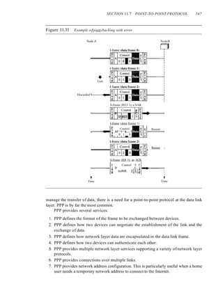
Example 11.10: Piggybacking without Error
Figure 11.30 shows an exchange using piggybacking. Node A begins the exchange of
information with an I-frame numbered 0 followed by another I-frame numbered 1. Node B
piggybacks its acknowledgment of both frames onto an I-frame of its own. Node B's first
I-frame is also numbered 0 [N(S) field] and contains a 2 in its N(R) field, acknowledging the
receipt of Ns frames 1 and 0 and indicating that it expects frame 2 to arrive next. Node B
transmits its second and third I-frames (numbered 1 and 2) before accepting further
frames from node A. Its N(R) information, therefore, has not changed: B frames 1 and 2
indicate that node B is still expecting Ns frame 2 to arrive next. Node A has sent all its
data. Therefore, it cannot piggyback an acknowledgment onto an I-frame and sends an S-frame
instead. The RR code indicates that A is still ready to receive. The number 3 in the N(R) field
tells B that frames 0, 1, and 2 have all been accepted and that A is now expecting frame
number 3.](https://image.slidesharecdn.com/cnforouzan4e-231013053408-7d177071/85/CN_Forouzan4e-pdf-382-320.jpg)


![356 CHAPTER 11 DATA LINK CONTROL
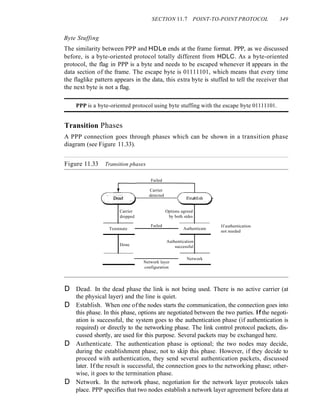
Figure 11.41 An example
User
[I
~
System
i
. Configure-request
~ Options
. LeI'
Authenticate-ack
§ITIr] Name
PAP
Authenticate-request
C023- ~ Name O-P-a-ss-w-o-rd-I
PAP
Configure-request·:
gOZL~ Options
IPCp·
Terminate-request
. CQ21:- ~ Options
LCP
[
y
Time
y
Time](https://image.slidesharecdn.com/cnforouzan4e-231013053408-7d177071/85/CN_Forouzan4e-pdf-393-320.jpg)
![SECTION 11.9 KEY TERMS 357
The first two frames show link establishment. We have chosen two options (not shown in the
figure): using PAP for authentication and suppressing the address control fields. Frames 3 and 4
are for authentication. Frames 5 and 6 establish the network layer connection using IPCP.
The next several frames show that some IP packets are encapsulated in the PPP frame. The
system (receiver) may have been running several network layer protocols, but it knows that the
incoming data must be delivered to the IP protocol because the NCP protocol used before the data
transfer was IPCP.
After data transfer, the user then terminates the data link connection, which is acknowledged
by the system. Of COUrse the user or the system could have chosen to terminate the network layer
IPCP and keep the data link layer running if it wanted to run another NCP protocol.
The example is trivial, but it points out the similarities of the packets in LCP, AP, and
NCP. It also shows the protocol field values and code numbers for particular protocols.
11.8 RECOMMENDED READING
For more details about subjects discussed in this chapter, we recommend the following
books. The items in brackets [...] refer to the reference list at the end of the text.
Books
A discussion of data link control can be found in [GW04], Chapter 3 of [Tan03], Chapter 7
of [Sta04], Chapter 12 of [Kes97], and Chapter 2 of [PD03]. More advanced materials can
be found in [KMK04].
11.9 KEY TERMS
acknowledgment (ACK)
asynchronous balanced mode (ABM)
automatic repeat request (ARQ)
bandwidth-delay product
bit-oriented protocol
bit stuffing
byte stuffing
Challenge Handshake Authentication
Protocol (CHAP)
character-oriented protocol
data link control
error control
escape character (ESC)
event
fixed-size framing
flag
flow control
framing
Go-Back-N ARQ Protocol
High-level Data Link Control (HDLC)
information frame (I-frame)
Internet Protocol Control Protocol (IPCP)
Link Control Protocol (LCP)
negative acknowledgment (NAK)
noiseless channel
noisy channel
normal response mode (NRM)
Password Authentication Protocol (PAP)
piggybacking
pipelining
Point-to-Point Protocol (PPP)
primary station](https://image.slidesharecdn.com/cnforouzan4e-231013053408-7d177071/85/CN_Forouzan4e-pdf-394-320.jpg)


![SECTION 12.1 RANDOM ACCESS 365
The random access methods we study in this chapter have evolved from a very
interesting protocol known as ALOHA, which used a very simple procedure called
multiple access (MA). The method was improved with the addition of a procedure that
forces the station to sense the medium before transmitting. This was called carrier sense
multiple access. This method later evolved into two parallel methods: carrier sense
multiple access with collision detection (CSMAlCD) and carrier sense multiple access
with collision avoidance (CSMA/CA). CSMA/CD tells the station what to do when a
collision is detected. CSMA/CA tries to avoid the collision.
ALOHA
ALOHA, the earliest random access method, was developed at the University of Hawaii
in early 1970. It was designed for a radio (wireless) LAN, but it can be used on any
shared medium.
It is obvious that there are potential collisions in this arrangement. The medium is
shared between the stations. When a station sends data, another station may attempt to
do so at the same time. The data from the two stations collide and become garbled.
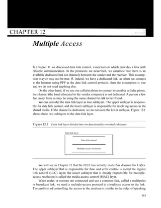
Pure ALOHA
The original ALOHA protocol is called pure ALOHA. This is a simple, but elegant
protocol. The idea is that each station sends a frame whenever it has a frame to send.
However, since there is only one channel to share, there is the possibility of collision
between frames from different stations. Figure 12.3 shows an example of frame collisions
in pure ALOHA.
Figure 12.3 Frames in a pure ALOHA network
[J
Station 1 ~I Frame 1.1 1 JFrame 1.21 ~
Time
[J
Station 2 ~ JFrame 2.1 L -' Frame 2.2 L ~
Time
[]
Station 3 ~ -1 Frame3.1 1 JFrame 3.2 I__ ~
Time
[]
Station 4 ~ J Frame4.1 L J Frame4.21 ~
Time
Collision
duration
Collision
duration
There are four stations (unrealistic assumption) that contend with one another for
access to the shared channel. The figure shows that each station sends two frames; there
are a total of eight frames on the shared medium. Some of these frames collide because
multiple frames are in contention for the shared channel. Figure 12.3 shows that only](https://image.slidesharecdn.com/cnforouzan4e-231013053408-7d177071/85/CN_Forouzan4e-pdf-402-320.jpg)
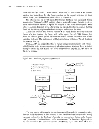
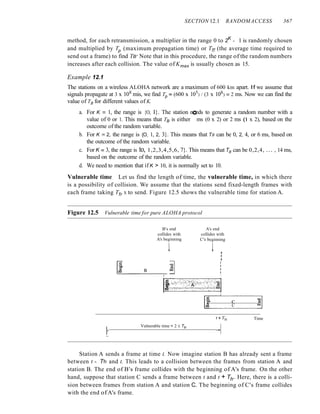

![SECTION /2.1 RANDOM ACCESS 369
Slotted ALOHA
Pure ALOHA has a vulnerable time of 2 x Tfr . This is so because there is no rule that
defines when the station can send. A station may send soon after another station has
started or soon before another station has finished. Slotted ALOHA was invented to
improve the efficiency of pure ALOHA.
In slotted ALOHA we divide the time into slots of Tfr s and force the station to
send only at the beginning of the time slot. Figure 12.6 shows an example of frame
collisions in slotted ALOHA.
Figure 12.6 Frames in a slotted ALOHA network
Collision Collision
duration duration
[J
Station] ~_ Frame 1.] Frame 1.2
-------------- ------ ---~
Time
Station 2
- Frame 2.1 Frame 2.2
-: ------ --,....--- ------ ------ ---+
Time
a--
Station 3 Frame 3.1 Frame 3.2
------ ...,,_ ....._-- ------- ------- ---~
Time
&--
Station 4 Frame 4.1 Frame 4.2
------ .....,_ ...... _--- ------ ------ ---~
Time
Slot 1 510t2 Slot 3 510t4 Slot 5 Slot 6
Because a station is allowed to send only at the beginning of the synchronized time
slot, if a station misses this moment, it must wait until the beginning of the next time
slot. This means that the station which started at the beginning of this slot has already
finished sending its frame. Of course, there is still the possibility of collision if two sta-
tions try to send at the beginning of the same time slot. However, the vulnerable time is
now reduced to one-half, equal to Tfr Figure 12.7 shows the situation.
Figure 12.7 shows that the vulnerable time for slotted ALOHA is one-half that of
pure ALOHA.
Slotted ALOHA vulnerable time = Tfr
Throughput It can be proved that the average number of successful transmissions for
slotted ALOHA is S = G x e-G
. The maximum throughput Smax is 0.368, when G = 1.
In other words, if a frame is generated during one frame transmission time, then 36.8
percent of these frames reach their destination successfully. This result can be expected
because the vulnerable time is equal to the frame transmission time. Therefore, if a sta-
tion generates only one frame in this vulnerable time (and no other station generates a
frame during this time), the frame will reach its destination successfully.
The throughput for slotted ALOHA is S =: G x e-G.
The maximum throughput Smax == 0.368 when G =1.](https://image.slidesharecdn.com/cnforouzan4e-231013053408-7d177071/85/CN_Forouzan4e-pdf-406-320.jpg)
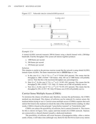
![SECTION 12.1 RANDOMACCESS 371
Figure 12.8 Space/time model ofthe collision in CSMA
B starts
at time 11
C starts
at time 12
Area where
A's signal exists
Area where
both signals exist
Time Time
and for every station to sense it. In other words, a station may sense the medium and find
it idle, only because the first bit sent by another station has not yet been received.
At time tI' station B senses the medium and finds it idle, so it sends a frame. At time
t2 (t2> tI)' station C senses the medium and finds it idle because, at this time, the first
bits from station B have not reached station C. Station C also sends a frame. The two
signals collide and both frames are destroyed.
Vulnerable Time
The vulnerable time for CSMA is the propagation time Tp . This is the time needed for
a signal to propagate from one end of the medium to the other. When a station sends a
frame, and any other station tries to send a frame during this time, a collision will
result. But if the first bit of the frame reaches the end of the medium, every station will
already have heard the bit and will refrain from sending. Figure 12.9 shows the worst
Figure 12.9 Vulnerable time in CSMA
B senses
here
Ill~~~~~~~
Frame propagation
Time
]
Vulnerable time
propagation time
Time](https://image.slidesharecdn.com/cnforouzan4e-231013053408-7d177071/85/CN_Forouzan4e-pdf-408-320.jpg)
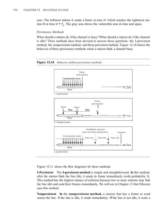


![SECTION 12.1 RANDOMACCESS 375
Figure 12.13 Collision and abortion in CSMAlCD
Collision
Transmission [1[ ~~;!~~i~~i~~~~I~~~~112 ]~ransmission
tIme 13 tIme
t4*~~
A detects
collision and
aborts
Time
C detects
collision
and aborts Time
Example 12.5
A network using CSMA/CD has a bandwidth of 10 Mbps. If the maximum propagation time
(including the delays in the devices and ignoring the time needed to send a jamming signal, as we
see later) is 25.611S, what is the minimum size of the frame?
Solution
The frame transmission time is Tfr =2 x Tp =51.2 ~s. This means, in the worst case, a station
needs to transmit for a period of 51.2 ~s to detect the collision. The minimum size of the frame
is 10 Mbps x 51.2 !-ls =512 bits or 64 bytes. This is actually the minimum size of the frame for
Standard Ethernet, as we will see in Chapter 13.
Procedure
Now let us look at the flow diagram for CSMAlCD in Figure 12.14. It is similar to the
one for the ALOHA protocol, but there are differences.
The first difference is the addition of the persistence process. We need to sense the
channel before we start sending the frame by using one of the persistence processes we
discussed previously (nonpersistent, I-persistent, or p-persistent). The corresponding
box can be replaced by one of the persistence processes shown in Figure 12.11.
The second difference is the frame transmission. In ALOHA, we first transmit the
entire frame and then wait for an acknowledgment. In CSMA/CD, transmission and
collision detection is a continuous process. We do not send the entire frame and then
look for a collision. The station transmits and receives continuously and simultaneously
(using two different ports). We use a loop to show that transmission is a continuous
process. We constantly monitor in order to detect one of two conditions: either trans-
mission is finished or a collision is detected. Either event stops transmission. When we
come out of the loop, if a collision has not been detected, it means that transmission is
complete; the entire frame is transmitted. Otherwise, a collision has occurred.
The third difference is the sending of a short jamming signal that enforces the colli-
sion in case other stations have not yet sensed the collision.
Energy Level
We can say that the level of energy in a channel can have three values: zero, normal,
and abnormal. At the zero level, the channel is idle. At the normal level, a station has](https://image.slidesharecdn.com/cnforouzan4e-231013053408-7d177071/85/CN_Forouzan4e-pdf-412-320.jpg)


![SECTION 12.3 CHANNELIZATION 387
2. If we multiply a sequence by a number, every element in the sequence is multiplied
by that element. This is called multiplication of a sequence by a scalar. For example,
2. [+1 +1-1-1]=[+2+2-2-2]
3. If we multiply two equal sequences, element by element, and add the results, we
get N, where N is the number of elements in the each sequence. This is called the
inner product of two equal sequences. For example,
[+1 +1-1 -n· [+1 +1 -1 -1] = 1 + 1 + 1 + 1 = 4
4. If we multiply two different sequences, element by element, and add the results,
we get O. This is called inner product of two different sequences. For example,
[+1 +1 -1 -1] • [+1 +1 +1 +1] = 1 + 1- 1- 1 = 0
5. Adding two sequences means adding the corresponding elements. The result is
another sequence. For example,
[+1+1-1-1]+[+1+1+1+1]=[+2+2 00]
Data Representation
We follow these rules for encoding: If a station needs to send a 0 bit, it encodes it as -1;
if it needs to send a 1 bit, it encodes it as +1. When a station is idle, it sends no signal,
which is interpreted as a O. These are shown in Figure 12.25.
Figure 12.25 Data representation in CDMA
I Data bit 0 --.~ -I II Data bit I ----1.~ +1 I! Silence ----I.~ 0 I
Encoding and Decoding
As a simple example, we show how four stations share the link during a I-bit interval.
The procedure can easily be repeated for additional intervals. We assume that stations 1
and 2 are sending a 0 bit and channel 4 is sending a 1 bit. Station 3 is silent. The data at
the sender site are translated to -1, -1, 0, and +1. Each station multiplies the correspond-
ing number by its chip (its orthogonal sequence), which is unique for each station. The
result is a new sequence which is sent to the channel. For simplicity, we assume that all
stations send the resulting sequences at the same time. The sequence on the channel is
the sum of all four sequences as defined before. Figure 12.26 shows the situation.
Now imagine station 3, which we said is silent, is listening to station 2. Station 3 mul-
tiplies the total data on the channel by the code for station 2, which is [+1 -1 +1-1], to get
[-1-1-3 +1]· [+1-1 +1-1] =-4/4 =-1 ...... bit 1](https://image.slidesharecdn.com/cnforouzan4e-231013053408-7d177071/85/CN_Forouzan4e-pdf-424-320.jpg)
![388 CHAPTER 12 MULTIPLE ACCESS
Figure 12.26 Sharing channel in CDMA
Bit a Bit a
C1
1+1 +1 +1 +IJ
d1
• c1
[-1 -I -I -I]
C2
1+1 -I +1 -1]
[-1 -1 -3 +1]
Data
Common
channel
c.-
[+1 +1 -1 -11
C4
1+1 -I -1 +11
Silent Bit 1
Signal Level
The process can be better understood if we show the digital signal produced by each
station and the data recovered at the destination (see Figure 12.27). The figure shows the
corresponding signals for each station (using NRZ-L for simplicity) and the signal that
is on the common channel.
Figure 12.27 Digital signal created by four stations in CDMA
BitO ~ 1-1 -1 -I -I]
BitO ~ 1-1 +1 -I +1]
Silent ~ [0 0 0 0]
Bit I ~ 1+1 -I -I +1]
Data on the channel
Time
Time
Time
Time
Time
Figure 12.28 shows how station 3 can detect the data sent by station 2 by using the
code for station 2. The total data on the channel are multiplied (inner product opera-
tion) by the signal representing station 2 chip code to get a new signal. The station then
integrates and adds the area under the signal, to get the value -4, which is divided by 4
and interpreted as bit O.](https://image.slidesharecdn.com/cnforouzan4e-231013053408-7d177071/85/CN_Forouzan4e-pdf-425-320.jpg)
![SECTION 12.3 CHANNELIZATION 389
Figure 12.28 Decoding ofthe composite signal for one in CDMA
Data on the channel
Time
Station 2's code
m [+1 -I +1 -1]
Inner product result
Summing the values
Time
Time
Time
-4 ~ -4/4 ~ -I ~ BitO
Sequence Generation
To generate chip sequences, we use a Walsh table, which is a two-dimensional table with
an equal number of rows and columns, as shown in Figure 12.29.
Figure 12.29 General rule and examples ofcreating Walsh tables
a. Two basic rules
WI = [+1 J +1 +1 +1 +1
+1 -1 +1 -1
W4 =
[+1 +1J +1 +1 -1 -1
Wz =
+1 -1 +1 -1 -1 +1
b. Generation of WI' Wz,and W4
In the Walsh table, each row is a sequence of chips. WI for a one-chip sequence has
one row and one column. We can choose -lor +1 for the chip for this trivial table (we
chose +1). According to Walsh, if we know the table for N sequences WN' we can create
the table for 2N sequences W2N, as shown in Figure 12.29. The WN with the overbar WN
stands for the complement of WN' where each +1 is changed to -1 and vice versa.
Figure 12.29 also shows how we can create W2 and W4 from WI' After we select WI, W2](https://image.slidesharecdn.com/cnforouzan4e-231013053408-7d177071/85/CN_Forouzan4e-pdf-426-320.jpg)
![390 CHAPTER 12 MULTIPLE ACCESS
can be made from four Wj 's, with the last one the complement of Wl' After W2 is gener-
ated, W4 can be made of four W2's, with the last one the complement of W2. Of course,
Ws is composed of four W4's, and so on. Note that after WN is made, each station is
assigned a chip corresponding to a row.
Something we need to emphasize is that the number of sequences N needs to be a
power of 2. In other words, we need to have N = 2m.
The number of sequences in a Walsh table needs to beN = 2m.
Example 12.6
Find the chips for a network with
a. Two stations
b. Four stations
Solution
We can use the rows of W2 and W4 in Figure 12.29:
a. For a two-station network, we have [+1 +1] and [+1-1].
b. For a four-station network we have [+1 +1 +1 +1], [+1 -1 +1 -1], [+1 +1 -1 -1], and
[+1-1-1 +1].
Example 12.7
What is the number of sequences if we have 90 stations in our network?
Solution
The number of sequences needs to be 2m
. We need to choose m = 7 and N = 27
or 128. We can
then use 90 of the sequences as the chips.
Example 12.8
Prove that a receiving station can get the data sent by a specific sender if it multiplies the entire
data on the channel by the sender's chip code and then divides it by the number of stations.
Solution
Let us prove this for the first station, using our previous four-station example. We can say that the
data on the channel D =Cdl . ("1 + d2 . ("2 + d3 . ("3 + d4 . ("4)' The receiver which wants to get the
data sent by station I multiplies these data by ("I'
D . ("1 =(d1 • ("1 + d2 . ("2 + d3 . ("3 + d4 . ("4) . ("1
= d1 . ("1 . ("1 + d2 . ("2 . ("1 + d3 . ("3 . ("1 + d4 . ("4 . ("1
=d I X N + d2 X 0 +d3 X 0 + d4 X 0
=dl xN
When we divide the result by N, we get dI'
12.4 RECOMMENDED READING
For more details about subjects discussed in this chapter, we recommend the following
books. The items in brackets [...Jrefer to the reference list at the end of the text.](https://image.slidesharecdn.com/cnforouzan4e-231013053408-7d177071/85/CN_Forouzan4e-pdf-427-320.jpg)
![SECTION 12.6 SUMMARY 391
Books
Multiple access is discussed in Chapter 4 of [Tan03], Chapter 16 of [Sta04], Chapter 6 of
[GW04], and Chapter 8 of [For03]. More advanced materials can be found in [KMK04].
12.5 KEY TERMS
I-persistent method
ALOHA
binary exponential backup
carrier sense multiple access (CSMA)
carrier sense multiple access with
collision avoidance (CSMAlCA)
carrier sense multiple access with
collision detection (CSMAlCD)
channelization
code-division multiple access (CDMA)
collision
contention
controlled access
frequency-division multiple access
(FDMA)
inner product
interframe space (IFS)
jamming signal
multiple access (MA)
nonpersistent method
orthogonal sequence
polling
p-persistent method
primary station
propagation time
pure ALOHA
random access
reservation
secondary station
slotted ALOHA
time-division multiple access
(TDMA)
token
token passing
vulnerable time
Walsh table
12.6 SUMMARY
o We can consider the data link layer as two sublayers. The upper sublayer is responsible
for data link control, and the lower sublayer is responsible for resolving access to the
shared media.
U Many formal protocols have been devised to handle access to a shared link. We cate-
gorize them into three groups: random access protocols, controlled access protocols,
and channelization protocols.
o In random access or contention methods, no station is superior to another station
and none is assigned the control over another.
o ALOHA allows multiple access (MA) to the shared medium.There are potential
collisions in this arrangement. When a station sends data, another station may attempt
to do so at the same time. The data from the two stations collide and become garbled.
o To minimize the chance of collision and, therefore, increase the performance, the
CSMA method was developed. The chance of collision can be reduced if a station](https://image.slidesharecdn.com/cnforouzan4e-231013053408-7d177071/85/CN_Forouzan4e-pdf-428-320.jpg)

![SECTION 12.7 PRACTICE SET 393
3. Define controlled access and list three protocols in this category.
4. Define channelization and list three protocols in this category.
5. Explain why collision is an issue in a random access protocol but not in controlled
access or channelizing protocols.
6. Compare and contrast a random access protocol with a controlled access protocol.
7. Compare and contrast a random access protocol with a channelizing protocol.
8. Compare and contrast a controlled access protocol with a channelizing protocol.
9. Do we need a multiple access protocol when we use the 1ocalloop of the telephone
company to access the Internet? Why?
10. Do we need a multiple access protocol when we use one CATV channel to access
the Internet? Why?
Exercises
11. We have a pure ALOHA network with 100 stations. If Tfr = 1 }.is, what is the number
of frames/s each station can send to achieve the maximum efficiency.
12. Repeat Exercise 11 for slotted ALOHA.
13. One hundred stations on a pure ALOHA network share a l-Mbps channel. If frames
are 1000 bits long, find the throughput if each station is sending 10 frames per
second.
14. Repeat Exercise 13 for slotted ALOHA.
15. In a CDMAlCD network with a data rate of 10 Mbps, the minimum frame size is
found to be 512 bits for the correct operation of the collision detection process. What
should be the minimum frame size if we increase the data rate to 100 Mbps? To
1 Gbps? To 10 Gbps?
16. In a CDMAlCD network with a data rate of 10 Mbps, the maximum distance
between any station pair is found to be 2500 m for the correct operation of the col-
lision detection process. What should be the maximum distance if we increase the
data rate to 100 Mbps? To 1 Gbps? To 10 Gbps?
17. In Figure 12.12, the data rate is 10 Mbps, the distance between station A and C is
2000 m, and the propagation speed is 2 x 10⁸
mls. Station A starts sending a long
frame at time t1 =0; station C starts sending a long frame at time t2 =3 }.is. The
size of the frame is long enough to guarantee the detection of collision by both
stations. Find:
a. The time when station C hears the collision (t3)'
b. The time when station A hears the collision (t4)'
c. The number of bits station A has sent before detecting the collision.
d. The number of bits station C has sent before detecting the collision.
18. Repeat Exercise 17 if the data rate is 100 Mbps.
19. Calculate the Walsh table Wsfrom W4 in Figure 12.29.
20. Recreate the W2 and W4 tables in Figure 12.29 using WI = [-1]. Compare the recre-
ated tables with the ones in Figure 12.29.
21. Prove the third and fourth orthogonal properties ofWalsh chips for W4 in Figure 12.29.](https://image.slidesharecdn.com/cnforouzan4e-231013053408-7d177071/85/CN_Forouzan4e-pdf-430-320.jpg)


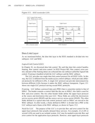


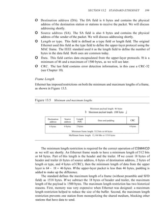


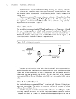
![SECTION 13.2 STANDARD ETHERNET 405
Figure 13.12 IOBase-T implementation
~OBr'Q
10 Mbps Twisted pair
Baseband
(digital)
iI~I
m iTwo pairs of
~ ~UTPcable
I[Q] [QJ ... ~I
lOBase-T hub
cable as far as a collision is concerned. The maximum length of the twisted cable here
is defined as 100 m, to minimize the effect of attenuation in the twisted cable.
lOBase-F: Fiber Ethernet
Although there are several types of optical fiber lO-Mbps Ethernet, the most common is
called 10Base-F. lOBase-F uses a star topology to connect stations to a hub. The stations
are connected to the hub using two fiber-optic cables, as shown in Figure 13.13.
Figure 13.13 IOBase-F implementation
~OBr~
]0 Mbps Fiber
Baseband
(digital)
lOBase-F hub
Two fiber-optic
cables
Summary
Table 13.1 shows a summary of Standard Ethernet implementations.
Table 13.1 Summary ofStandard Ethernet implementations
Characteristics lOBase5 lOBase2 lOBase-T IOBase-F
Media Thick Thin 2UTP 2 Fiber
coaxial cable coaxial cable
Maximum length 500m 185 m 100m 2000m
Line encoding Manchester Manchester Manchester Manchester](https://image.slidesharecdn.com/cnforouzan4e-231013053408-7d177071/85/CN_Forouzan4e-pdf-442-320.jpg)
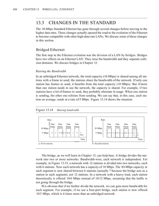


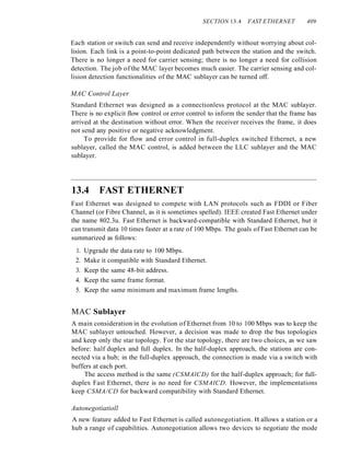


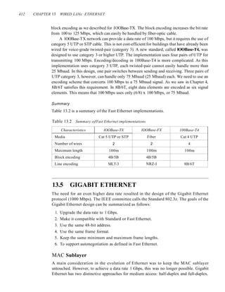

![414 CHAPTER 13 WIRED LANs: ETHERNET
Physical Layer
The physical layer in Gigabit Ethernet is more complicated than that in Standard or Fast
Ethernet. We briefly discuss some features of this layer.
Topology
Gigabit Ethernet is designed to connect two or more stations. If there are only two sta-
tions, they can be connected point-to-point. Three or more stations need to be connected
in a star topology with a hub or a switch at the center. Another possible configuration is
to connect several star topologies or let a star topology be part of another as shown in
Figure 13.22.
Figure 13.22 Topologies ofGigabit Ethernet
a-a
a. Point-to-point
ffi·
r~ r
="""":. = '""":. ="""':.
c. Two stars
d. Hierarchy of stars
ffi
r j r 3
=. roul;:;;:;]",": =-:.
Implementation
Gigabit Ethernet can be categorized as either a two-wire or a four-wire implementation.
The two-wire implementations use fiber-optic cable (1000Base-SX, short-wave, or
lOOOBase-LX, long-wave), or STP (1000Base-CX). The four-wire version uses cate-
gory 5 twisted-pair cable (lOOOBase-T). In other words, we have four implementations,
as shown in Figure 13.23. lOOOBase-T was designed in response to those users who](https://image.slidesharecdn.com/cnforouzan4e-231013053408-7d177071/85/CN_Forouzan4e-pdf-451-320.jpg)
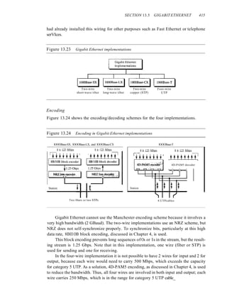
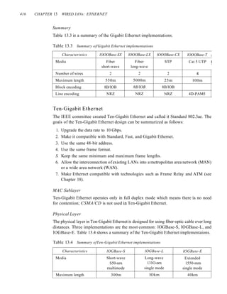
![SECTION 13.8 SUMMARY 417
13.6 RECOMMENDED READING
For more details about subjects discussed in this chapter, we recommend the following
books. The items in brackets [...] refer to the reference list at the end of the text.
Books
Ethernet is discussed in Chapters 10, 11, and 12 of [For03], Chapter 5 of [Kei02], Sec-
tion 4.3 of [Tan03], and Chapters 15 and 16 of [Sta04]. [SpuOO] is a book about Ethernet.
A complete discussion of Gigabit Ethernet can be found in [KCK98] and [Sau98].
Chapter 2 of [IzzOO] has a good comparison between different generations of Ethernet.
13.7 KEY TERMS
1000Base-CX
1000Base-LX
1000Base-SX
1000Base-T
100Base-FX
100Base-T4
100Base-TX
10Base2
lOBase5
lOBase-F
10Base-T
10GBase-E
lOGBase-L
10GBase-S
autonegotiation
bridge
carrier extension
Cheapernet
collision domain
destination service access point (DSAP)
Fast Ethernet
frame bursting
full-duplex switched Ethernet
Gigabit Ethernet
hexadecimal notation
logical link control (LLC)
media access control (MAC)
network interface card (NIC)
preamble
Project 802
source service access point (SSAP)
Standard Ethernet
switch
switched Ethernet
Ten-Gigabit Ethernet
thick Ethernet
Thicknet
thin Ethernet
transceiver
twisted-pair Ethernet
13.8 SUMMARY
o Ethernet is the most widely used local area network protocoL
o The IEEE 802.3 Standard defines I-persistent CSMA/CD as the access method for
first-generation 10-Mbps Ethernet.
o The data link layer of Ethernet consists of the LLC sublayer and the MAC sublayer.](https://image.slidesharecdn.com/cnforouzan4e-231013053408-7d177071/85/CN_Forouzan4e-pdf-454-320.jpg)


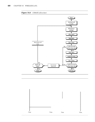


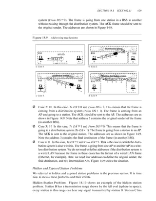
![430 CHAPTER 14 WIRELESS LANs
Figure 14.10 Hidden station problem
Range
ofB
(]
~
B
&
c
Range
ofC
Band Care hiddent from each other with respect to A.
a transmission range shown by the right oval (sphere in space); every station located
in this range can hear any signal transmitted by C. Station C is outside the transmis-
sion range of B; likewise, station B is outside the transmission range of C. Station A,
however, is in the area covered by both Band C; it can hear any signal transmitted by
B or C.
Assume that station B is sending data to station A. In the middle ofthis transmission,
station C also has data to send to station A. However, station C is out of B's range and
transmissions from B cannot reach C. Therefore C thinks the medium is free. Station C
sends its data to A, which results in a collision at A because this station is receiving data
from both B and C. In this case, we say that stations Band C are hidden from each other
with respect to A. Hidden stations can reduce the capacity of the network because of the
possibility of collision.
The solution to the hidden station problem is the use of the handshake frames (RTS
and CTS) that we discussed earlier. Figure 14.11 shows that the RTS message from B
reaches A, but not C. However, because both Band C are within the range of A, the
CTS message, which contains the duration of data transmission from B to A reaches C.
Station C knows that some hidden station is using the channel and refrains from trans-
mitting until that duration is over.
The CTS frame in CSMAICA handshake can prevent collision
from a hidden station.
Figure 14.11 Use ofhandshaking to prevent hidden station problem
B A C
r
CTS CTS
Time Time Time](https://image.slidesharecdn.com/cnforouzan4e-231013053408-7d177071/85/CN_Forouzan4e-pdf-467-320.jpg)

![125
MHz
432 CHAPTER i4 WiRELESS LANs
Physical Layer
We discuss six specifications, as shown in Table 14.4.
Table 14.4 Physical layers
IEEE Technique Band Modulation Rate (Mbps)
802.11 FHSS 2.4 GHz FSK 1 and 2
DSSS 2.4 GHz PSK 1 and 2
Infrared PPM 1 and 2
802.11a OFDM 5.725 GHz PSKorQAM 6 to 54
802.l1b DSSS 2.4 GHz PSK 5.5 and 11
802.1Ig OFDM 2.4 GHz Different 22 and 54
All implementations, except the infrared, operate in the industrial, scientific,
and medical (ISM) band, which defines three unlicensed bands in the three ranges
902-928 MHz, 2.400--4.835 GHz, and 5.725-5.850 GHz, as shown in Figure 14.14.
Figure 14.14 industrial, scient(fic, and medical (ISM) band
26 83.5
,MHz, MHz, ,
~ ~I.----'JI 1:1( "I
, ",.-----' '=.,.....--~--...,.,,'
~
'kV ; I'~:£--:} 0 0_. . .:,,,,:,].
~;~~ ~~:-
<3A> ,i1."< 1...- ----l.. I:.::;.:;.-l~--.:...~:::~-'~,L;~J
'0-'.
'.:...'.':.....'....:.,-"--"..:.....0....... '- ~.
902 928 2.4 2.4835 5.725 5.850 Frequency
MHz MHz GHz GHz GHz GHz
IEEE 802.11 FHSS
IEEE 802.11 FHSS uses the frequency-hopping spread spectrum (FHSS) method as
discussed in Chapter 6. FHSS uses the 2.4-GHz ISM band. The band is divided into
79 subbands of 1 MHz (and some guard bands). A pseudorandom number generator
selects the hopping sequence. The modulation technique in this specification is either
two-level FSK or four-level FSK with I or 2 bitslbaud, which results in a data rate of 1
or 2 Mbps, as shown in Figure 14.15.
IEEE 802.11 DSSS
IEEE 802.11 DSSS uses the direct sequence spread spectrum (DSSS) method as dis-
cussed in Chapter 6. DSSS uses the 2.4-GHz ISM band. The modulation technique in this
specification is PSK at 1Mbaud/s. The system allows 1 or 2 bitslbaud (BPSK or QPSK),
which results in a data rate of 1 or 2 Mbps, as shown in Figure 14.16.
IEEE 802.11 Infrared
IEEE 802.11 infrared uses infrared light in the range of 800 to 950 nm. The modulation
technique is called pulse position modulation (PPM). For a I-Mbps data rate, a 4-bit](https://image.slidesharecdn.com/cnforouzan4e-231013053408-7d177071/85/CN_Forouzan4e-pdf-469-320.jpg)
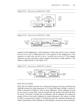

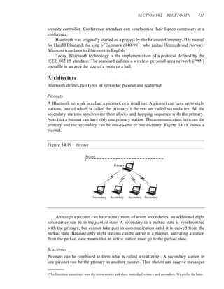
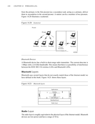

![fO
438 CHAPTER 14 WIRELESS LANs
In slot 0, the primary sends, and the secondary receives; in slot 1, the secondary sends, and
the primary receives. The cycle is repeated. Figure 14.22 shows the concept.
Figure 14.22 Single-secondary communication
I 625 Jls I
i ' ~ i
I, .1 I
: 366 Jls I : I I
r-rr---:----i Hop I r-rr---l Hop:
Primary -+LL---JL...----;i--------lI-LL-----JL...----+,------+---l.~
l
it 1 I Time
, I: ii,
Secondary ~----_crr=J_H_O_P--l:----~OCJ_H-O-p_+i ---l'~
I I I I Time
I fl ! f2 ! f3 !
Multiple-Secondary Communication The process is a little more involved if there is
more than one secondary in the piconet. Again, the primary uses the even-numbered slots,
but a secondary sends in the next odd-numbered slot if the packet in the previous slot was
addressed to it. All secondaries listen on even-numbered slots, but only one secondary
sends in any odd-numbered slot. Figure 14.23 shows a scenario.
Figure 14.23 Multiple-secondary communication
I I I I
-OCJHOP
: CIT=]Hop !
•
Primary I
j
I
1
I Time
I I
I I
I I
I I
I I
I I
I I
I
Hop I
Secondary 1
I
I Time
I
I
I
I
I
I
I
Secondary 2
trr=JHOp
•
I
I
f3
Time
fO fl f2 J
Let us elaborate on the figure.
1. In slot 0, the primary sends a frame to secondary 1.
2. In slot 1, only secondary I sends a frame to the primary because the previous frame
was addressed to secondary 1; other secondaries are silent.](https://image.slidesharecdn.com/cnforouzan4e-231013053408-7d177071/85/CN_Forouzan4e-pdf-475-320.jpg)


![SECTION 14.3 RECOMMENDED READING 441
Figure 14.25 L2CAP data packetfarmat
2 bytes 2 bytes 0 to 65,535 bytes
Length I Channel ID 1 D_at_a_an_d_co_n_tro_l _
Multiplexing
The L2CAP can do multiplexing. At the sender site, it accepts data from one of the
upper-layer protocols, frames them, and delivers them to the baseband layer. At the
receiver site, it accepts a frame from the baseband layer, extracts the data, and delivers
them to the appropriate protocol layer. It creates a kind of virtual channel that we will
discuss in later chapters on higher-level protocols.
Segmentation and Reassembly
The maximum size of the payload field in the baseband layer is 2774 bits, or 343 bytes.
This includes 4 bytes to define the packet and packet length. Therefore, the size of the
packet that can arrive from an upper layer can only be 339 bytes. However, application
layers sometimes need to send a data packet that can be up to 65,535 bytes (an Internet
packet, for example). The L2CAP divides these large packets into segments and adds
extra information to define the location of the segments in the original packet. The
L2CAP segments the packet at the source and reassembles them at the destination.
QoS
Bluetooth allows the stations to define a quality-of-service level. We discuss quality of
service in Chapter 24. For the moment, it is sufficient to know that if no quality-of-service
level is defined, Bluetooth defaults to what is called best-effort service; it will do its best
under the circumstances.
Group Management
Another functionality of L2CAP is to allow devices to create a type of logical addressing
between themselves. This is similar to multicasting. For example, two or three secondary
devices can be part of a multicast group to receive data from the primary.
Other Upper Layers
Bluetooth defines several protocols for the upper layers that use the services of L2CAP;
these protocols are specific for each purpose.
14.3 RECOMMENDED READING
For more details about subjects discussed in this chapter, we recommend the follow-
ing books and sites. The items in brackets [...] refer to the reference list at the end of
the text.](https://image.slidesharecdn.com/cnforouzan4e-231013053408-7d177071/85/CN_Forouzan4e-pdf-478-320.jpg)
![442 CHAPTER 14 WIRELESS LANs
Books
Wireless LANs and Bluetooth are discussed in several books including [Sch03] and
[Gas02]. Wireless LANs are discussed in Chapter 15 of [For03], Chapter 17 of [Sta04],
Chapters 13 and 14 of [Sta02], and Chapter 8 of [Kei021. Bluetooth is discussed in
Chapter 15 of [Sta02] and Chapter 15 of [For03].
14.4 KEY TERMS
access point (AP)
asynchronous connectionless link
(ACL)
basic service set (BSS)
beacon frame
Bluetooth
BSS-transition mobility
complementary code keying (CCK)
direct sequence spread spectrum (OSSS)
distributed coordination function (OCF)
distributed interframe space (OIFS)
ESS-transition mobility
extended service set (ESS)
frequency-hopping spread spectrum
(FHSS)
handshaking period
high-rate direct sequence spread spectrum
(HR-OSSS)
IEEE 802.11
Logical Link Control and Adaptation
Protocol (L2CAP)
network allocation vector (NAV)
no-transition mobility
orthogonal frequency-division
multiplexing (OFOM)
piconet
point coordination function (PCF)
primary
pulse position modulation (PPM)
repetition interval
scatternet
secondary
short interframe space (SIFS)
synchronous connection-oriented
(SCO)
TDD-TOMA (time-division duplex
TOMA)
wireless LAN
14.5 SUMMARY
o The IEEE 802.11 standard for wireless LANs defines two services: basic service
set (BSS) and extended service set (ESS).
o The access method used in the distributed coordination function (OCF) MAC sub-
layer is CSMAICA.
o The access method used in the point coordination function (PCF) MAC sublayer is
polling.
o The network allocation vector (NAV) is a timer used for collision avoidance.
o The MAC layer frame has nine fields. The addressing mechanism can include up to
four addresses.
o Wireless LANs use management frames, control frames, and data frames.](https://image.slidesharecdn.com/cnforouzan4e-231013053408-7d177071/85/CN_Forouzan4e-pdf-479-320.jpg)
![SECTION 14.6 PRACTICE SET 443
o IEEE 802.11 defines several physical layers, with different data rates and modulating
techniques.
o Bluetooth is a wireless LAN technology that connects devices (called gadgets) in a
small area.
o A Bluetooth network is called a piconet. Multiple piconets fonn a network called a
scatternet.
o A Bluetooth network consists of one primary device and up to seven secondary
devices.
14.6 PRACTICE SET
Review Questions
1. What is the difference between a BSS and an ESS?
2. Discuss the three types of mobility in a wireless LAN.
3. How is OFDM different from FDM?
4. What is the access method used by wireless LANs?
5. What is the purpose of the NAV?
6. Compare a piconet and a scatternet.
7. Match the layers in Bluetooth and the Internet model.
8. What are the two types of links between a Bluetooth primary and a Bluetooth
secondary?
9. In multiple-secondary communication, who uses the even-numbered slots and who
uses the odd-numbered slots?
10. How much time in a Bluetooth one-slot frame is used for the hopping mechanism?
What about a three-slot frame and a five-slot frame?
Exercises
1]. Compare and contrast CSMAlCD with CSMAICA.
12. Use Table 14.5 to compare and contrast the fields in IEEE 802.3 and 802.11.
Table 14.5 Exercise 12
Fields IEEE 802.3 Field Size IEEE 802.11 Field Size
Destination address
Source address
Address 1
Address 2
Address 3
Address 4
FC](https://image.slidesharecdn.com/cnforouzan4e-231013053408-7d177071/85/CN_Forouzan4e-pdf-480-320.jpg)


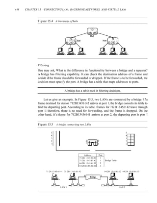
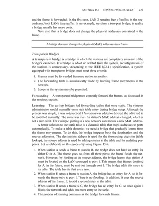
![450 CHAPTER 15 CONNECTING LANs, BACKBONE NETWORKS, AND VIRTUAL LANs
Figure 15.6 A learning bridge and the process oflearning
r-------JL------, 3
1--------1
LAN 2 D-'""'T"--"---'""'T"--c:;]
LAN 1 D-......I.--~-.....L._-c;;]
LAN 3
Address Port Address Port
A 1
Address Port
A 1
E 3
Address Port
A 1
E 3
B I
a. Original b. After A sends
a frame to D
c. After E sends
a frame to A
d. After B sends
a frame to C
Loop Problem Transparent bridges work fine as long as there are no redundant
bridges in the system. Systems administrators, however, like to have redundant bridges
(more than one bridge between a pair of LANs) to make the system more reliable. If a
bridge fails, another bridge takes over until the failed one is repaired or replaced.
Redundancy can create loops in the system, which is very undesirable. Figure 15.7
shows a very simple example of a loop created in a system with two LANs connected
by two bridges.
1. Station A sends a frame to station D. The tables of both bridges are empty. Both
forward the frame and update their tables based on the source address A.
2. Now there are two copies of the frame on LAN 2. The copy sent out by bridge 1 is
received by bridge 2, which does not have any information about the destination
address D; it floods the bridge. The copy sent out by bridge 2 is received by bridge 1
and is sent out for lack of information about D. Note that each frame is handled
separately because bridges, as two nodes on a network sharing the medium, use an
access method such as CSMA/CD. The tables of both bridges are updated, but still
there is no information for destination D.
3. Now there are two copies of the frame on LAN 1. Step 2 is repeated, and both copies
flood the network.
4. The process continues on and on. Note that bridges are also repeaters and regen-
erate frames. So in each iteration, there are newly generated fresh copies of the
frames.
To solve the looping problem, the IEEE specification requires that bridges use the
spanning tree algorithm to create a loopless topology.](https://image.slidesharecdn.com/cnforouzan4e-231013053408-7d177071/85/CN_Forouzan4e-pdf-487-320.jpg)

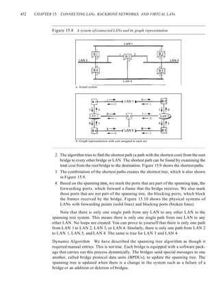


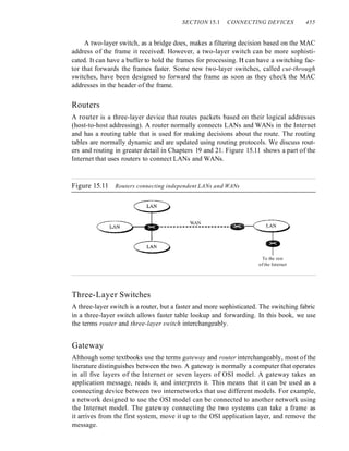

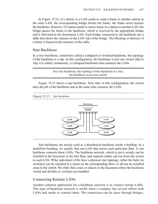


![SECTION 15.5 KEY7ERMS 463
Advantages
There are several advantages to using VLANs.
Cost and Time Reduction
VLANs can reduce the migration cost of stations going from one group to another.
Physical reconfiguration takes time and is costly. Instead of physically moving one sta-
tion to another segment or even to another switch, it is much easier and quicker to move
it by using software.
Creating Virtual Work Groups
VLANs can be used to create virtual work groups. For example, in a campus environ-
ment, professors working on the same project can send broadcast messages to one
another without the necessity of belonging to the same department. This can reduce
traffic if the multicasting capability of IP was previously used.
Security
VLANs provide an extra measure of security. People belonging to the same group can
send broadcast messages with the guaranteed assurance that users in other groups will
not receive these messages.
15.4 RECOMMENDED READING
For more details about subjects discussed in this chapter, we recommend the following
books and sites. The items in brackets [...] refer to the reference list at the end of the text.
Books
A book devoted to connecting devices is [PerOO]. Connecting devices and VLANs are
discussed in Section 4.7 of [Tan03]. Switches, bridges, and hubs are discussed in [Sta03]
and [Sta04].
Site
o IEEE 802 LAN/MAN Standards Committee
15.5 KEY TERMS
amplifier
blocking port
bridge
bus backbone
connecting device
filtering
forwarding port
hub
remote bridge
repeater
router
segment](https://image.slidesharecdn.com/cnforouzan4e-231013053408-7d177071/85/CN_Forouzan4e-pdf-500-320.jpg)


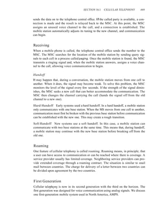


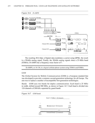
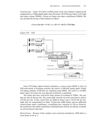


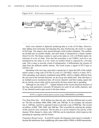


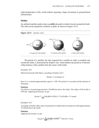


![SECTION 16.5 SUMMARY 487
at the corresponding time slot. The tenninal can send data during its time slot. A tenninal
receives all packets intended for the cell, but selects only those intended for its address.
Bands Transmission occurs in the Ka bands.
Data Rate The data rate is up to 155 Mbps for the uplink and up to 1.2 Gbps for the
downlink.
16.3 RECOMMENDED READING
For more details about subjects discussed in this chapter, we recommend the following
books. The items in brackets [...] refer to the reference list at the end of the text.
Books
Wireless WANs are completely covered in [Sta02], [Jam03], [AZ03], and [Sch03]. Com-
munication satellites are discussed in Section 2.4 of [Tan03] and Section 8.5 of [CouOl].
Mobile telephone system is discussed in Section 2.6 of [Tan03] and Section 8.8 of [CouOl].
16.4 KEY TERMS
Advanced Mobile Phone System (AMPS)
cellular telephony
digital AMPS (D-AMPS)
downlink
footprint
geostationary Earth orbit (GEO)
Global Positioning System (GPS)
Global System for Mobile
Communication (GSM)
Globalstar
handoff
Interim Standard 95 (IS-95)
Internet Mobile Communication 2000
(IMT-2000)
Iridium
low-Earth-orbit (LEO)
medium-Earth-orbit (MEO)
mobile switching center (MSC)
orbit
personal communications system
(PCS)
reuse factor
roamIng
satellite network
Teledesic
triangulation
trilateration
uplink
16.5 SUMMARY
o Cellular telephony provides communication between two devices. One or both may
be mobile.
o A cellular service area is divided into cells.
o Advanced Mobile Phone System (AMPS) is a first-generation cellular phone
system.](https://image.slidesharecdn.com/cnforouzan4e-231013053408-7d177071/85/CN_Forouzan4e-pdf-524-320.jpg)


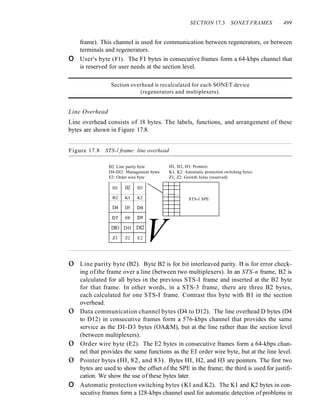
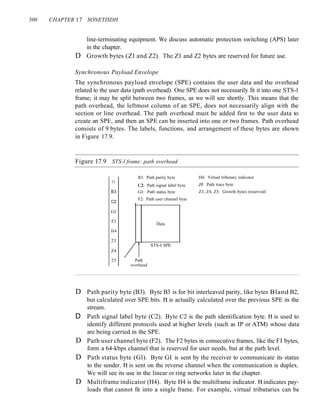


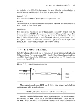
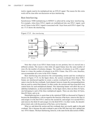

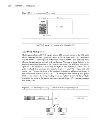

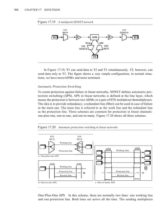

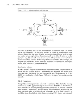


![SECTION 17.8 KEY TERMS 513
Figure 17.26 Virtual tributary types
VT1.5 =8000 frames/s 3 columns 9 rows 8 bits =1.728 Mbps
VT2 =8000 frames/s 4 columns 9 rows 8 bits = 2.304 Mbps
VT3 = 8000 frarnes/s 6 columns 9 rows 8 bits =3.456 Mbps
VT6 = 8000 frames/s 12 columns 9 rows 8 bits = 6.912 Mbps
VT1.5 VT2 VT3 VT6
When two or more tributaries are inserted into a single STS-1 frame. they are
interleaved column by column. SONET provides mechanisms for identifying each
VT and separating them without demultiplexing the entire stream. Discussion of
these mechanisms and the control issues behind them is beyond the scope of this
book.
17.7 RECOMMENDED READING
For more details about subjects discussed in this chapter, we recommend the following
books. The items in brackets [...] refer to the reference list at the end of the text.
Books
SONET is discussed in Section 2.5 of [Tan03], Section 15.2 of [Kes97], Sections 4.2
and 4.3 of [GW04], Section 8.2 of [Sta04], and Section 5.2 of [WVOOl
17.8 KEY TERMS
add/drop multiplexer (ADM)
automatic protection switching (APS)
bidirectional line switching ring (BLSR)
byte interleaving
line
line layer
line overhead (LOH)
optical carrier (Oe)
path
path layer
path overhead (POH)
photonic layer
regenerator
section
section layer
section overhead (SOH)
STS demultiplexer
STS multiplexer
Synchronous Digital Hierarchy (SDH)
Synchronous Optical Network (SONET)](https://image.slidesharecdn.com/cnforouzan4e-231013053408-7d177071/85/CN_Forouzan4e-pdf-550-320.jpg)
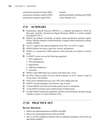


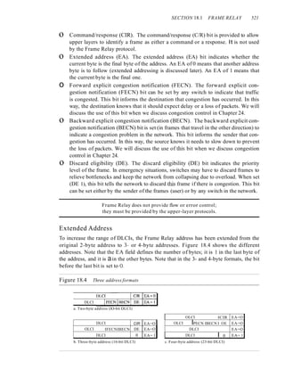
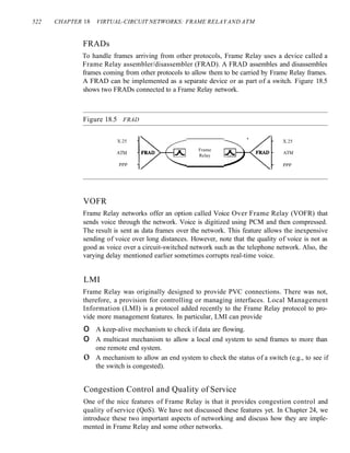


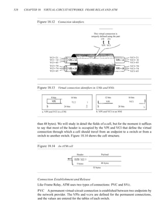
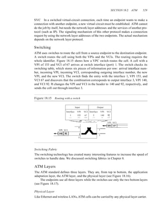

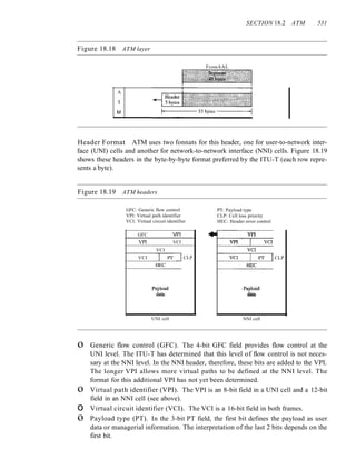


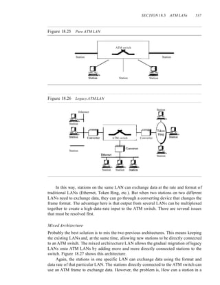
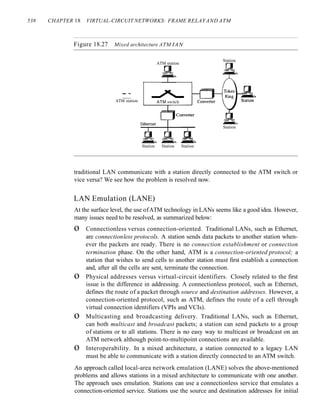


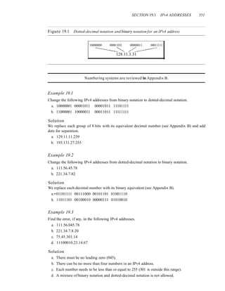


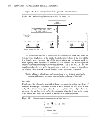

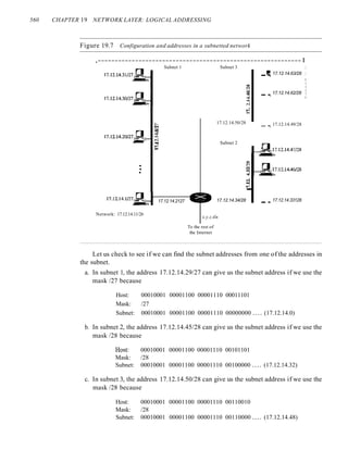


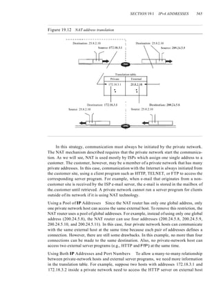
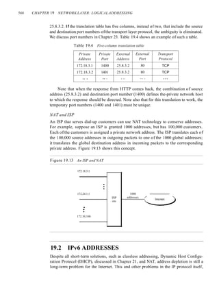


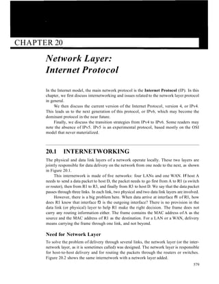


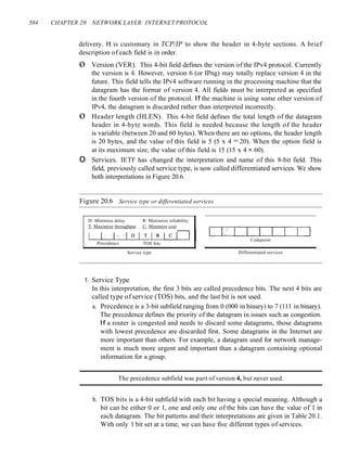
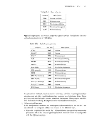


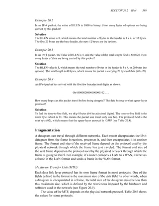
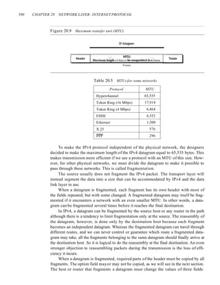
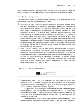

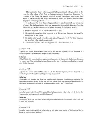


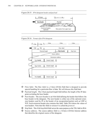


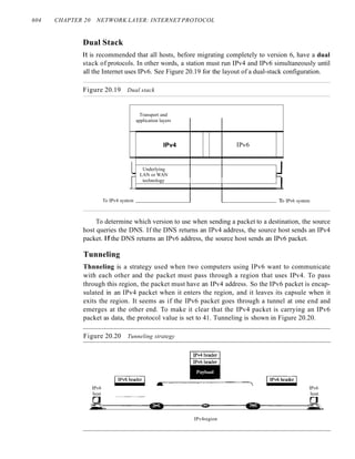


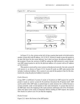


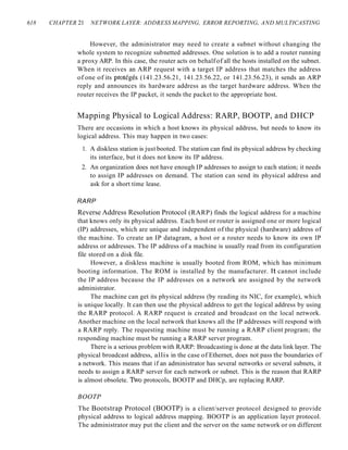
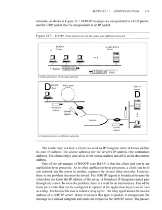


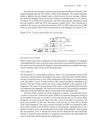

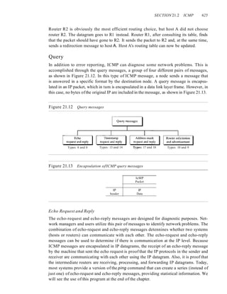


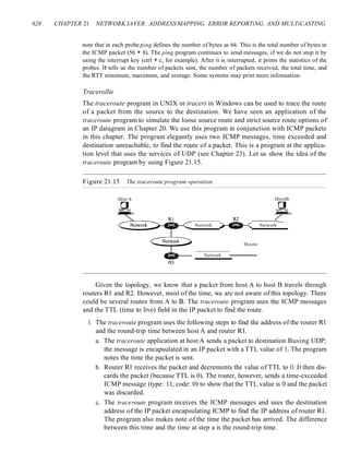


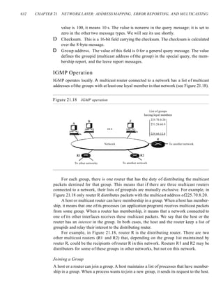


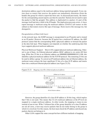


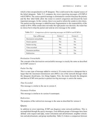


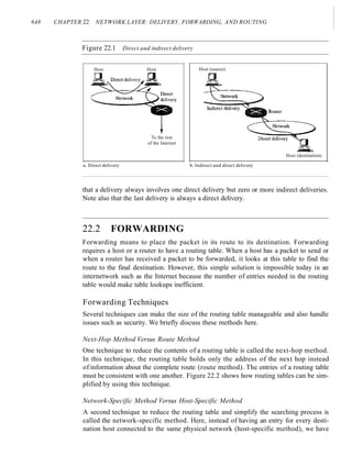
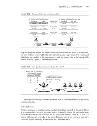
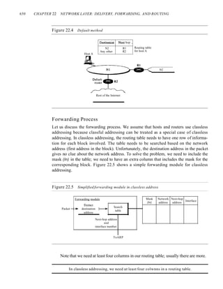


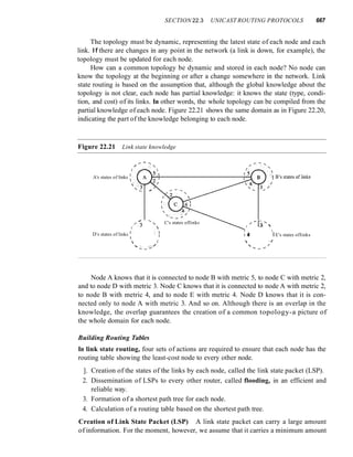
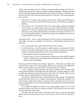
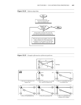


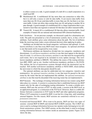
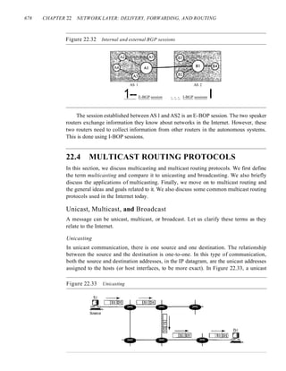


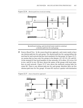

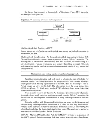


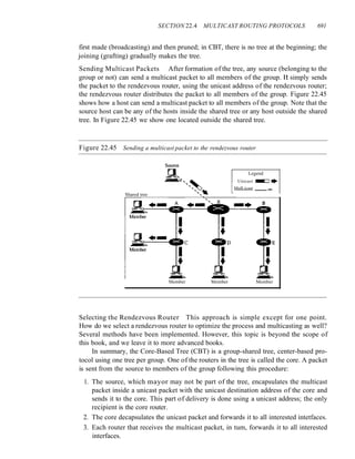


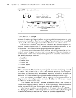
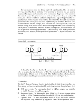
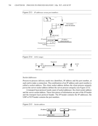


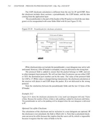


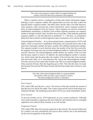


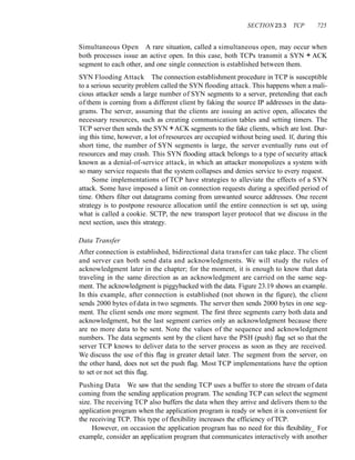
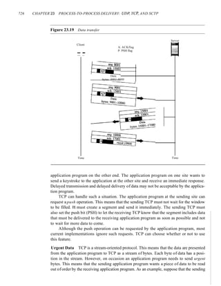
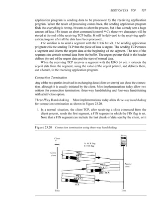

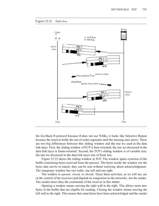
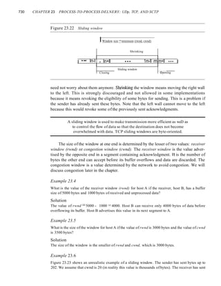
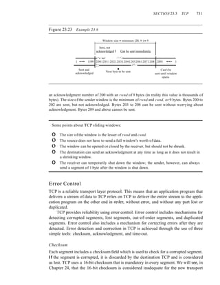

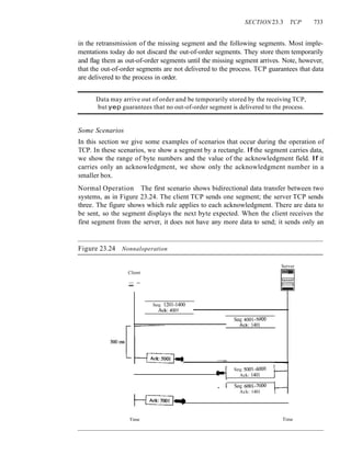
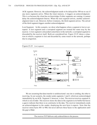
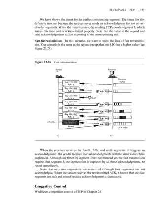


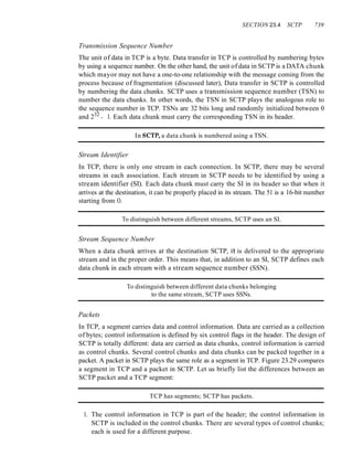


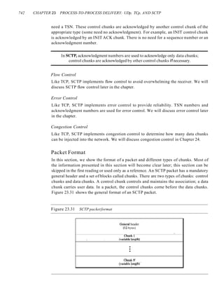
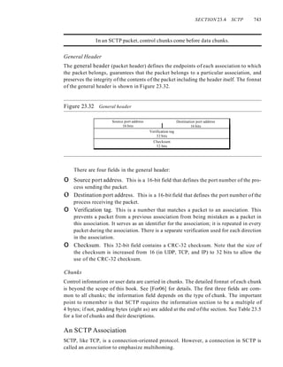

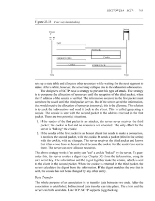

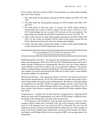


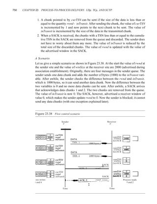


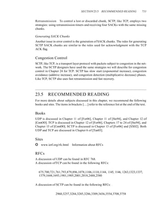


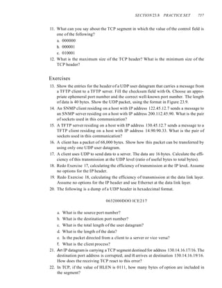


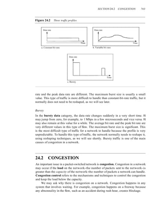


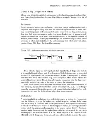
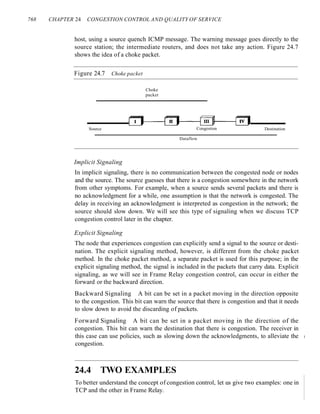


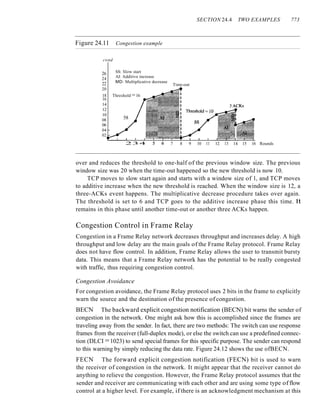


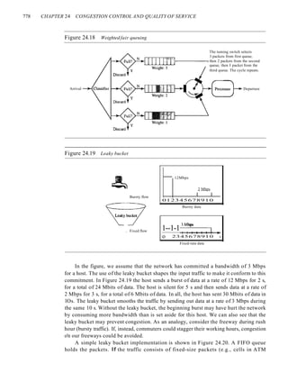


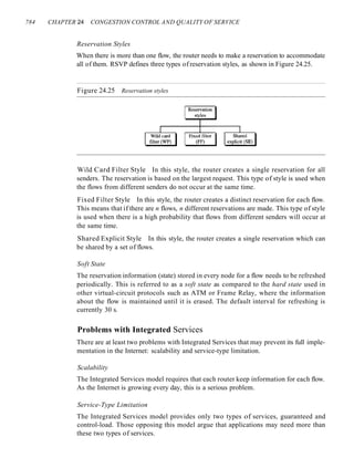


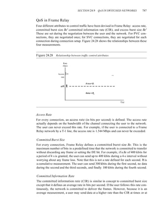
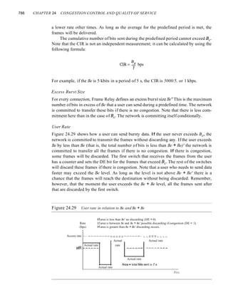


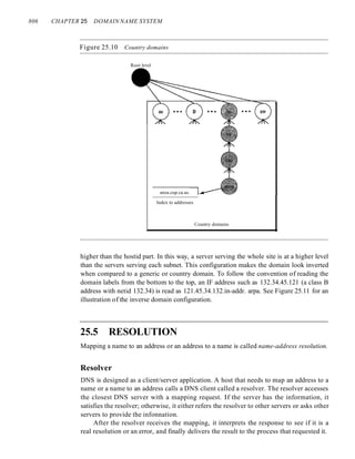
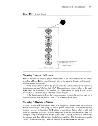


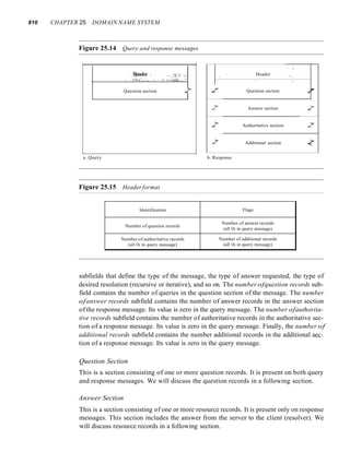


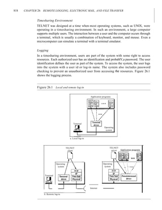
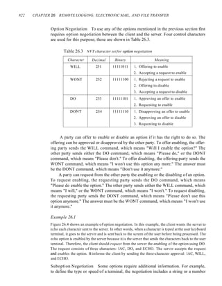


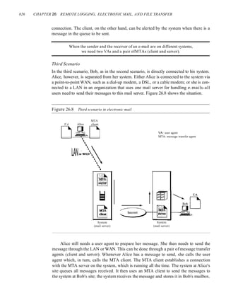


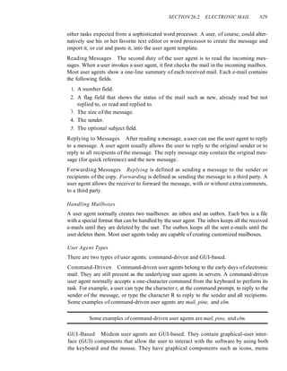
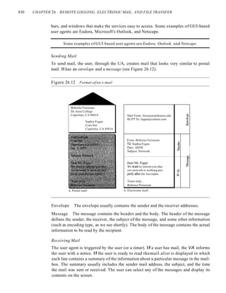
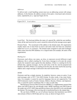

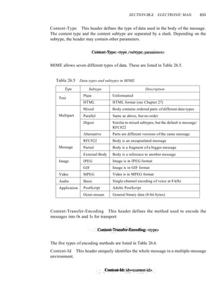


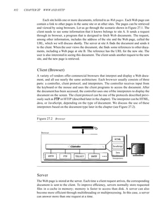
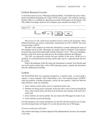


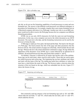

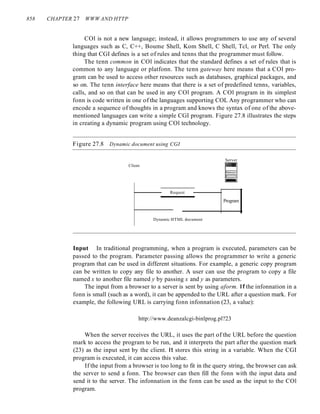
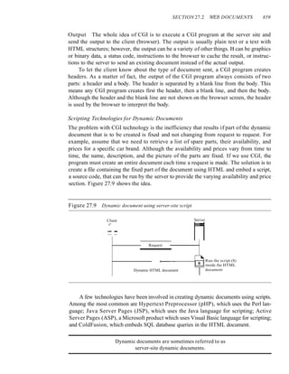
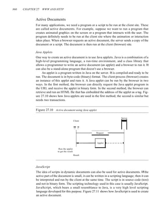
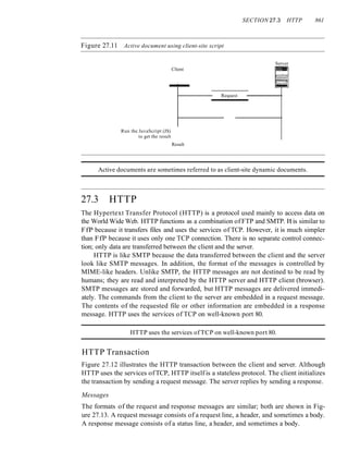
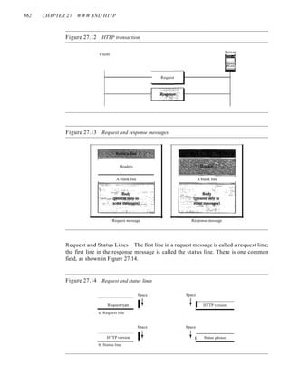
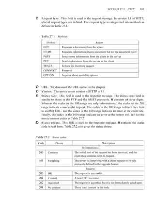
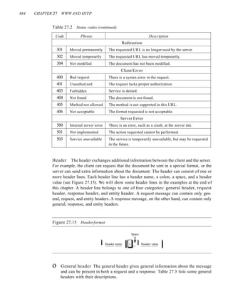
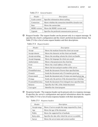
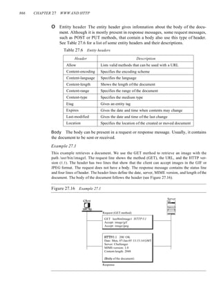


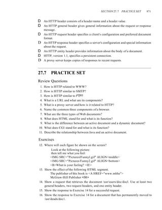


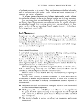

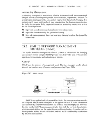


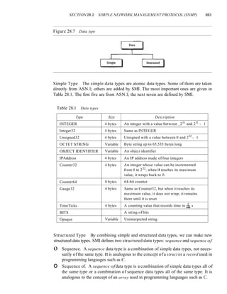
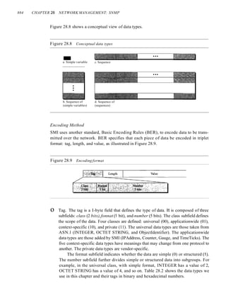
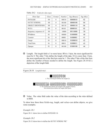


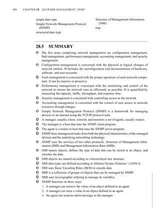


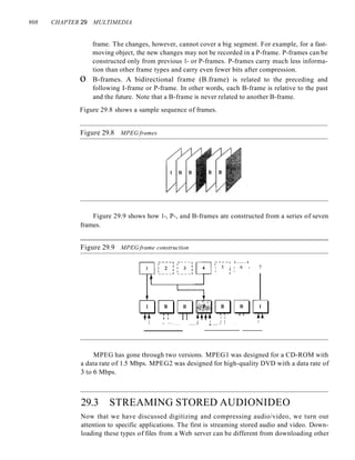


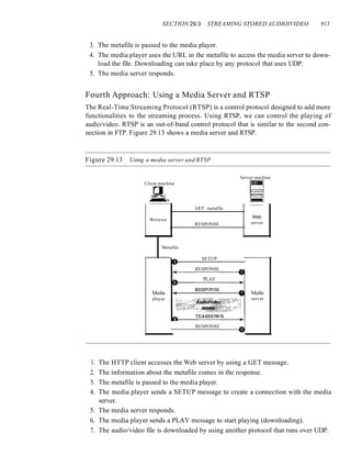
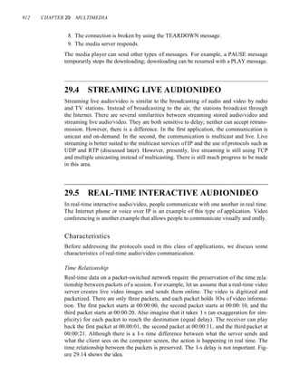


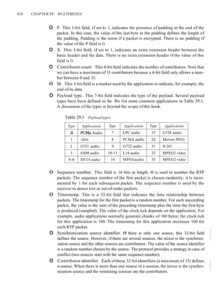


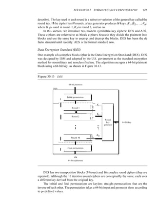
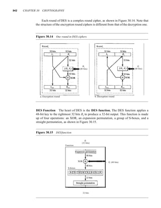
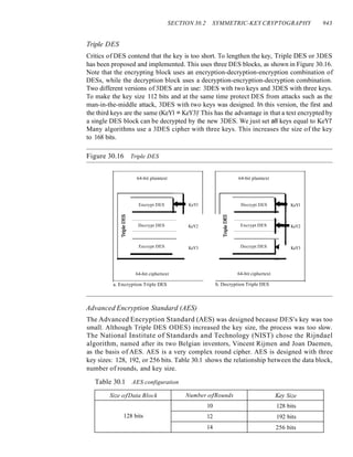


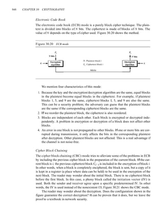

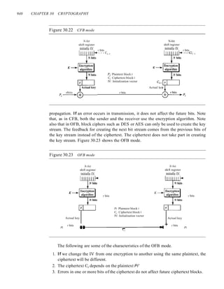


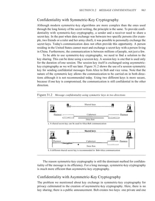

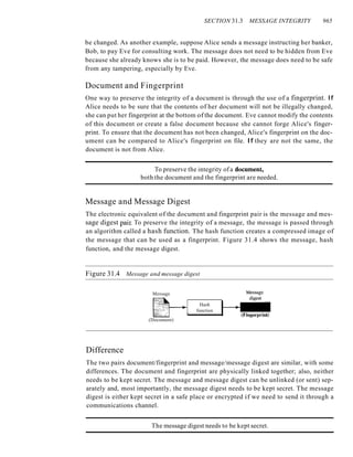
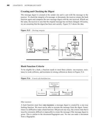


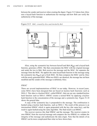


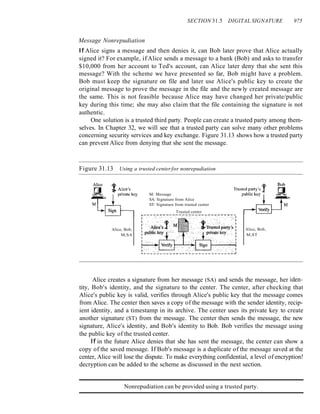


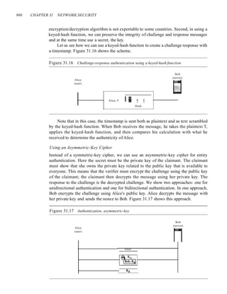


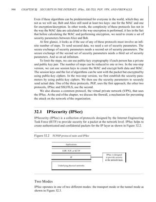

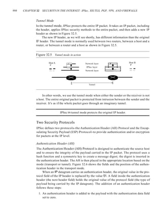

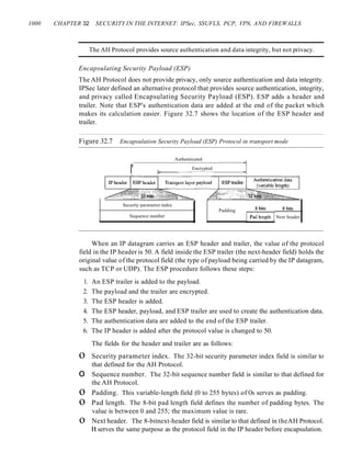


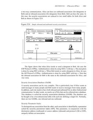


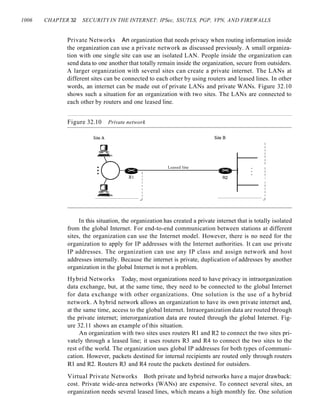
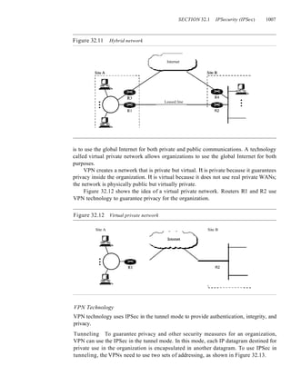


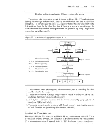

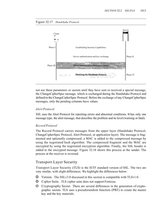


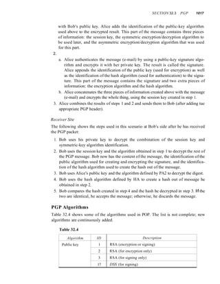
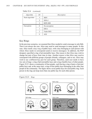


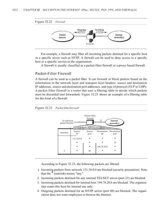


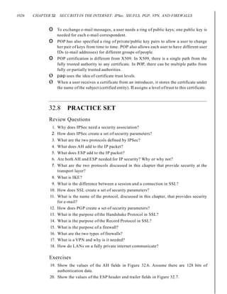


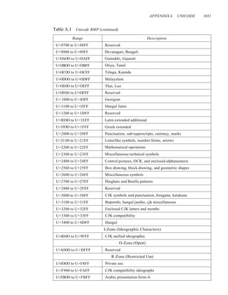


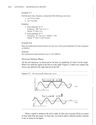


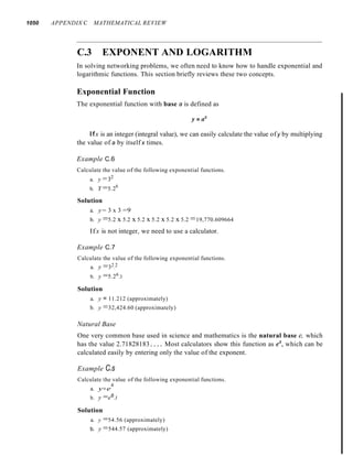


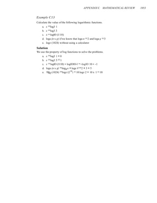


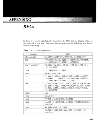

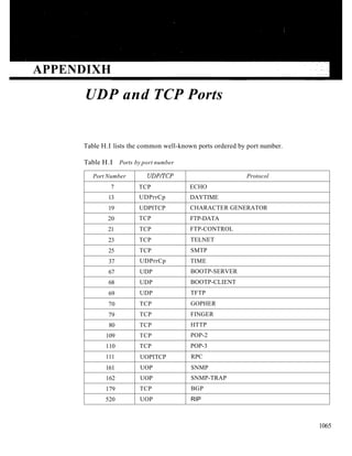


![01_-_W01L01_-_Introduction[1].pp free tx](https://cdn.slidesharecdn.com/ss_thumbnails/01-w01l01-introduction1-240627064011-cf787583-thumbnail.jpg?width=640&height=640&fit=bounds)