Download to read offline
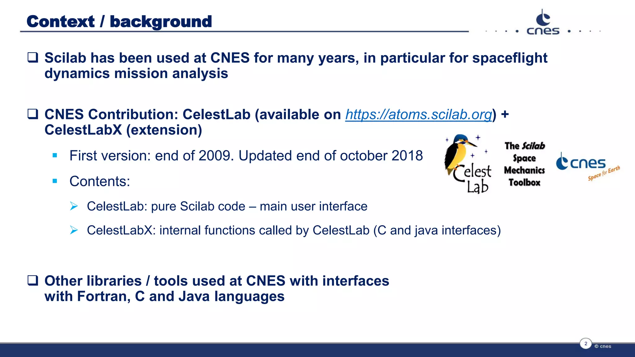
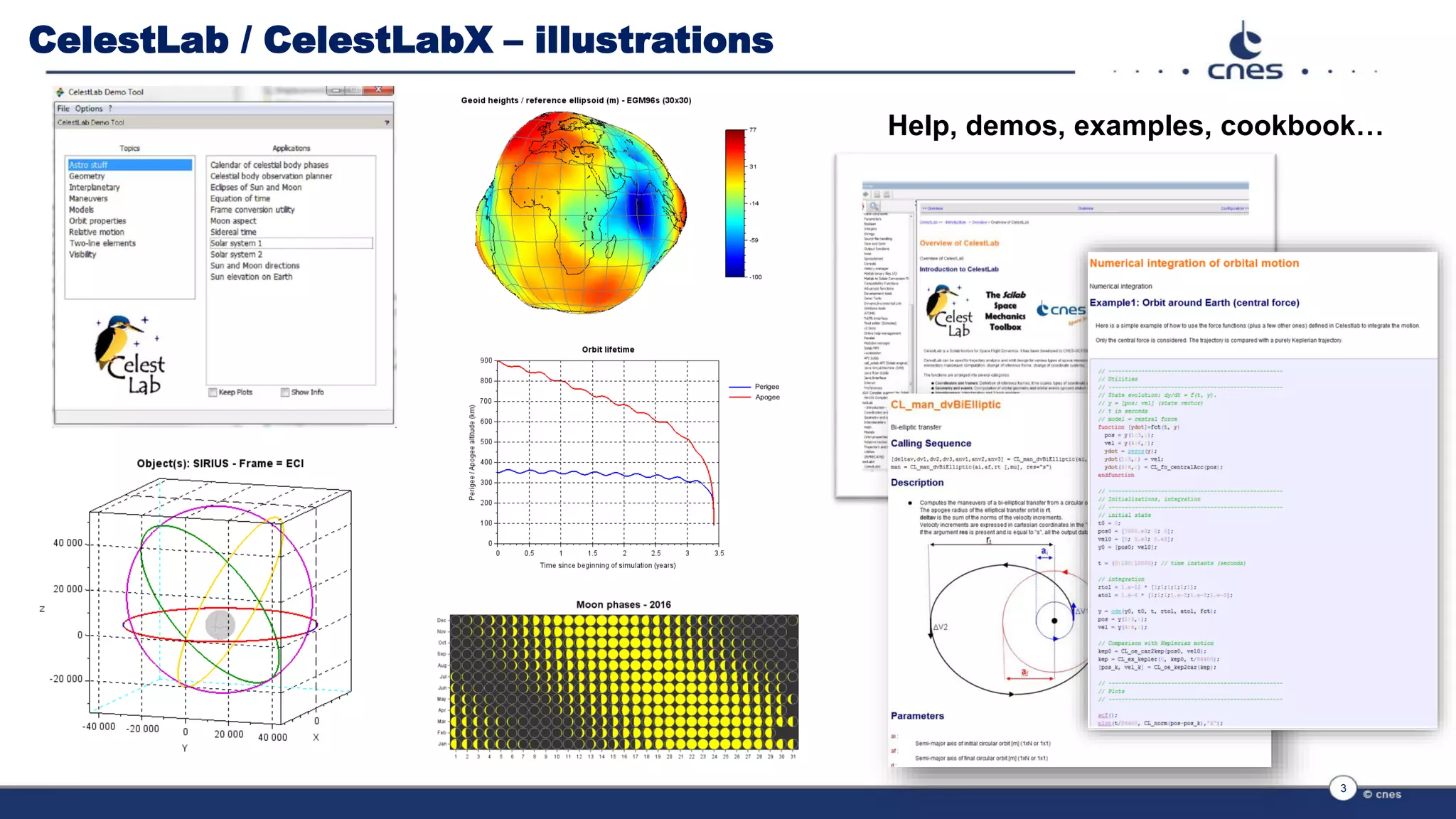
![Example of use of Java interface (STELA)
Example from Celestlab
// Initial date (time scale: TREF)
cjd0 = CL_dat_cal2jd(2018, 11, 16);
// Keplerian mean orbital elements (frame: ECI)
mean_kep0 = [7.e6; 1.e-3; 98*(%pi/180); %pi/2; 0; 0];
// Final dates
cjd = cjd0 + (0:60);
// STELA model parameters (default values)
params = CL_stela_params();
// Propagation
mean_kep = CL_stela_extrap("kep", cjd0, mean_kep0, cjd, params, "m");
// Plot inclination (deg)
scf();
plot(cjd – cjd0, mean_kep(3,:) * (180/%pi));
CL_g_stdaxes();
Structure of model parameters (forces…)
Initial state
Extrapolation dates
Easy to use
Looks like pure Scilab code
5](https://image.slidesharecdn.com/presentationscilabconference2018cneslamy-181128180251/75/CNES-Scilab-Conference-2018-5-2048.jpg)
![Numerical integration of orbital motion
Position = σ 𝒂𝒄𝒄𝒆𝒍𝒆𝒓𝒂𝒕𝒊𝒐𝒏
Several examples in CelestLab using ode
Rather straightforward, but the computation
of some forces can be very time consuming
=> slow execution
One possibility: interface functions written
in compiled languages
=> would imply lots of rewriting.
6
// Dynamic model
function [ydot]=fct(t, y)
pos = y(1:3,:);
vel = y(4:6,:);
ydot = zeros(y);
ydot(1:3,:) = vel;
ydot(4:6,:) = CL_fo_centralAcc(pos);
endfunction
// Initial state
t0 = 0;
y0 = [7.e6; 0; 0; 0; 7.e3; 0];
t = (0:180:10000); // time instants (seconds)
// Integration
rtol = 1.e-12 * [1;1;1;1;1;1];
atol = 1.e-6 * [1;1;1;1.e-3;1.e-3;1.e-3];
y = ode(y0, t0, t, rtol, atol, fct);](https://image.slidesharecdn.com/presentationscilabconference2018cneslamy-181128180251/75/CNES-Scilab-Conference-2018-6-2048.jpg)
![Basic example
Typical example (from function help)
8
// Initial orbit state (position/velocity, frame: CIRS, time scale: TREF)
cjd0 = CL_dat_cal2cjd(2004, 10, 4);
kep0 = [7.e6; 1.e-3; 98 * (%pi/180); 0; 0; 0];
pv0 = CL_oe_convert("kep", "pv", kep0);
// Epoch of final orbit states
cjd = cjd0 + (0 : 60 : 86400) / 86400;
// Model parameters (default values)
params = ms_orbp_params();
// Propagation
pv = ms_orbp_extrap(cjd0, pv0, cjd, params, "pv");
// Plot osculating semi-major axis and inclination
kep = CL_oe_convert("pv", "kep", pv);
scf();
plot(cjd, kep(1,:) / 1000);
xtitle("Semi major axis (km)");
Similar to STELA example
Looks like pure Scilab code
Easy to use](https://image.slidesharecdn.com/presentationscilabconference2018cneslamy-181128180251/75/CNES-Scilab-Conference-2018-8-2048.jpg)
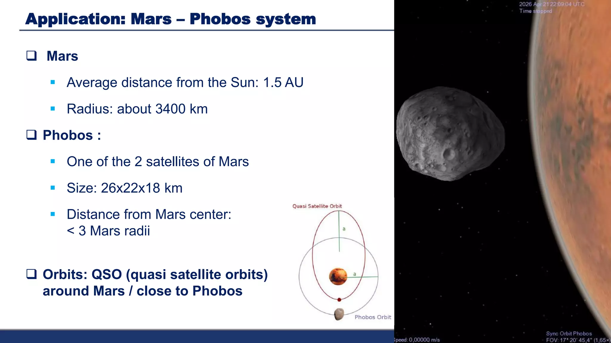

This document discusses interfacing Java code with Scilab for orbit propagation applications. It provides examples of using Java interfaces within Scilab code to perform orbit propagation in the Mars-Phobos system. The interfaces allow leveraging existing Java flight dynamics software for efficient numerical integration and propagation. The interfaces provide simple calls from Scilab that hide the complexity of the underlying Java code. The interfaces have been used successfully in studies of quasi-satellite orbits within the Mars-Phobos system.