The document discusses various topics related to cluster analysis, including:
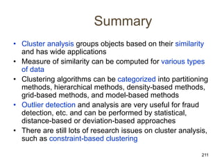
- What cluster analysis is and its typical applications
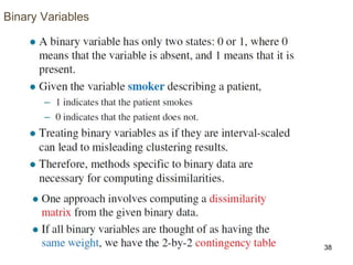
- The different types of data that can be used for cluster analysis, such as interval-scaled, binary, nominal, ordinal, and ratio variables
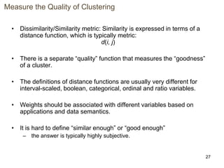
- The main stages of cluster analysis, including measuring the similarity or dissimilarity between objects, standardizing data, and measuring the quality of clustering results
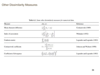
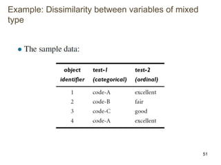
- Common methods for calculating the similarity or dissimilarity between different types of variables
The document provides an overview of cluster analysis, covering fundamental concepts and methods for handling different data types.