ML

1. * 1
SCSA1415
ML ESSENTIALS

2. * 2

3. 3

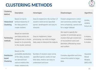
4. UNIT-III : CLUSTERING
* 4
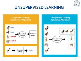
Clustering- K Means Clustering- Supervised
Learning after Clustering- Density Based Clustering
Methods- Hierarchical Based clustering methods-
Partitioning methods - Grid based methods.
Dimensionality Reduction : Linear Discriminant
Analysis - Principal Component Analysis.

5. UNSUPERVISED LEARNING
* 5

6. Clustering
• Clustering or cluster analysis is a machine learning technique,
which groups the unlabelled dataset.
• It can be defined as "A way of grouping the data points into
different clusters, consisting of similar data points. The
objects with the possible similarities remain in a group that
has less or no similarities with another group.“
• Finding some similar patterns in the unlabelled dataset such
as shape, size, color, behavior, etc., and divides them as per
the presence and absence of those similar patterns.
* 6

7. • It is an unsupervised learning method, hence no supervision is
provided to the algorithm, and it deals with the unlabeled
dataset.
• After applying this clustering technique, each cluster or group
is provided with a cluster-ID. ML system can use this id to
simplify the processing of large and complex datasets.
• The clustering technique is commonly used for statistical data
analysis.
Note: Clustering is somewhere similar to the classification algorithm, but the
difference is the type of dataset that we are using. In classification, we
work with the labeled data set, whereas in clustering, we work with the
unlabelled dataset.
* 7
Clustering

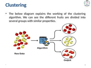
8. • The below diagram explains the working of the clustering
algorithm. We can see the different fruits are divided into
several groups with similar properties.
* 8
Clustering

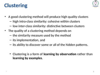
9. • A good clustering method will produce high quality clusters
– high intra-class similarity: cohesive within clusters
– low inter-class similarity: distinctive between clusters
• The quality of a clustering method depends on
– the similarity measure used by the method
– its implementation, and
– its ability to discover some or all of the hidden patterns.
• Clustering is a form of learning by observation rather than
learning by examples.
* 9
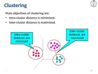
Clustering

10. Main objectives of clustering are:
• Intra-cluster distance is minimized.
• Inter-cluster distance is maximized.
* 10
Clustering

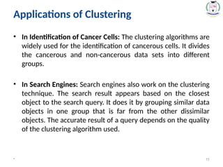
11. Applications of Clustering
• In Identification of Cancer Cells: The clustering algorithms are
widely used for the identification of cancerous cells. It divides
the cancerous and non-cancerous data sets into different
groups.
• In Search Engines: Search engines also work on the clustering
technique. The search result appears based on the closest
object to the search query. It does it by grouping similar data
objects in one group that is far from the other dissimilar
objects. The accurate result of a query depends on the quality
of the clustering algorithm used.
* 11

12. Applications of Clustering
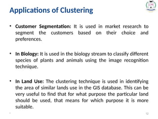
• Customer Segmentation: It is used in market research to
segment the customers based on their choice and
preferences.
• In Biology: It is used in the biology stream to classify different
species of plants and animals using the image recognition
technique.
• In Land Use: The clustering technique is used in identifying
the area of similar lands use in the GIS database. This can be
very useful to find that for what purpose the particular land
should be used, that means for which purpose it is more
suitable.
* 12

13. Applications of Clustering
•The clustering technique can be widely used in various tasks.
Some most common uses of this technique are:
– Market Segmentation
– Statistical data analysis
– Social network analysis
– Image segmentation
– Anomaly detection, etc.
•Apart from these general usages, it is used by the Amazon in its
recommendation system to provide the recommendations as per
the past search of products.
•Netflix also uses this technique to recommend the movies and
web-series to its users as per the watch history.
* 13

14. Data Matrix and Dissimilarity Matrix
* 14

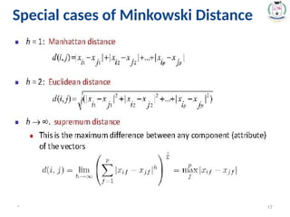
15. Similarity and Dissimilarity
• Distances are normally used to measure the similarity or
dissimilarity between to data objects.
• Some popular distances are based on Minkowski distance
(Lp or Lh norm)
* 15

16. * 16
Similarity and Dissimilarity

17. Special cases of Minkowski Distance
* 17

18. Example
* 18

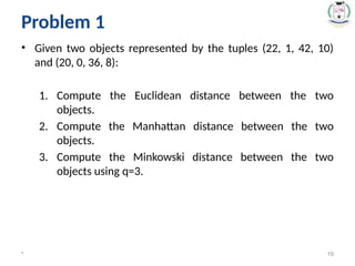
19. • Given two objects represented by the tuples (22, 1, 42, 10)
and (20, 0, 36, 8):
1. Compute the Euclidean distance between the two
objects.
2. Compute the Manhattan distance between the two
objects.
3. Compute the Minkowski distance between the two
objects using q=3.
* 19
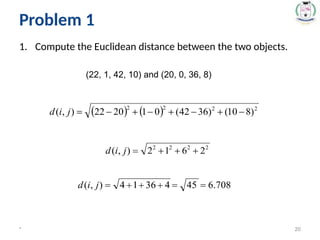
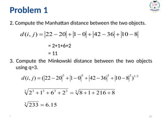
Problem 1

20. 1. Compute the Euclidean distance between the two objects.
* 20
(22, 1, 42, 10) and (20, 0, 36, 8)
Problem 1

21. 2. Compute the Manhattan distance between the two objects.
= 2+1+6+2
= 11
3. Compute the Minkowski distance between the two objects
using q=3.
* 21
Problem 1

22. Given 5-dimensional numeric samples A=(1,0,2,5,3) and
B=(2,1,0,3,-1).
1. Compute the Euclidean distance between the two
objects.
2. Compute the Manhattan distance between the two
objects.
3. Compute the Supremum distance.
* 22
Problem 2

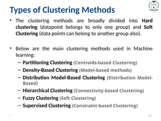
23. Types of Clustering Methods
• The clustering methods are broadly divided into Hard
clustering (datapoint belongs to only one group) and Soft
Clustering (data points can belong to another group also).
• Below are the main clustering methods used in Machine
learning:
– Partitioning Clustering (Centroids-based Clustering)
– Density-Based Clustering (Model-based methods)
– Distribution Model-Based Clustering (Distribution Model-
Based)
– Hierarchical Clustering (Connectivity-based Clustering)
– Fuzzy Clustering (Soft Clustering)
– Supervised Clustering (Constraint-based Clustering)
* 23

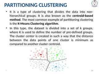
24. PARTITIONING CLUSTERING
• It is a type of clustering that divides the data into non-
hierarchical groups. It is also known as the centroid-based
method. The most common example of partitioning clustering
is the K-Means Clustering algorithm.
• In this type, the dataset is divided into a set of k groups,
where K is used to define the number of pre-defined groups.
The cluster center is created in such a way that the distance
between the data points of one cluster is minimum as
compared to another cluster centroid.
* 24

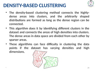
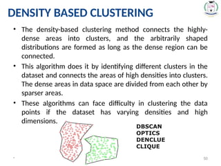
25. DENSITY-BASED CLUSTERING
• The density-based clustering method connects the highly-
dense areas into clusters, and the arbitrarily shaped
distributions are formed as long as the dense region can be
connected.
• This algorithm does it by identifying different clusters in the
dataset and connects the areas of high densities into clusters.
The dense areas in data space are divided from each other by
sparser areas.
• These algorithms can face difficulty in clustering the data
points if the dataset has varying densities and high
dimensions.
* 25

26. HIERARCHICAL CLUSTERING
• Hierarchical clustering can be used as an alternative for the
partitioned clustering as there is no requirement of pre-
specifying the number of clusters to be created.
• In this technique, the dataset is divided into clusters to create
a tree-like structure, which is also called a Dendrogram.
1. Top-down [Divisive Approach]
2. Bottom-up [Agglomerative Approach]
* 26

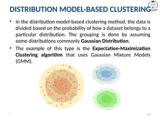
27. DISTRIBUTION MODEL-BASED CLUSTERING
• In the distribution model-based clustering method, the data is
divided based on the probability of how a dataset belongs to a
particular distribution. The grouping is done by assuming
some distributions commonly Gaussian Distribution.
• The example of this type is the Expectation-Maximization
Clustering algorithm that uses Gaussian Mixture Models
(GMM).
* 27

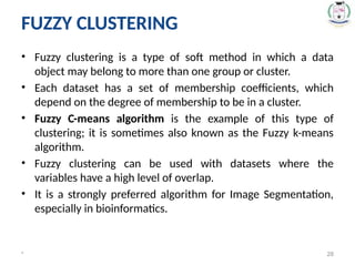
28. FUZZY CLUSTERING
• Fuzzy clustering is a type of soft method in which a data
object may belong to more than one group or cluster.
• Each dataset has a set of membership coefficients, which
depend on the degree of membership to be in a cluster.
• Fuzzy C-means algorithm is the example of this type of
clustering; it is sometimes also known as the Fuzzy k-means
algorithm.
• Fuzzy clustering can be used with datasets where the
variables have a high level of overlap.
• It is a strongly preferred algorithm for Image Segmentation,
especially in bioinformatics.
* 28

29. * 29
• In certain business scenarios, we might be required to
partition the data based on certain constraints.
• Here is where a supervised version of clustering machine
learning techniques come into play.
• A constraint is defined as the desired properties of the
clustering results, or a user’s expectation on the clusters.
• This can be in terms of a fixed number of clusters, or, the
cluster size, or, important dimensions (variables) that are
required for the clustering process.
• Usually, tree-based, Classification machine learning
algorithms like Decision Trees, Random Forest, and Gradient
Boosting, etc. are made use of to attain constraint-based
clustering.
SUPERVISED CLUSTERING

30. • Given a database of n objects or data tuples , a partitioning
method constructs k partitions of the data , where each
partition represents a cluster and k<=n.
• k is the number of groups after the classification of objects.
There are some requirements which need to be satisfied with
this Partitioning Clustering Method :
– Each group must contain at least one object
– Each object must belong to exactly one group.
* 30
PARTITIONING CLUSTERING METHOD

31. • Technique named Iterative Relocation is employed, which
means the object will be moved from one group to another to
improve the partitioning.
• The general criterion of a good partitioning is that object in
the same clusters are “close” or related to each other ,
whereas objects of different clusters are “far apart” or very
different.
• Example:
– K-MEANS, K--MEDIODS ,CLARANS
* 31
PARTITIONING CLUSTERING METHOD

32. PARTITION BASED CLUSTERING
* 32

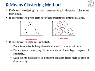
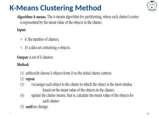
33. K-Means Clustering Method
• K-Means clustering is an unsupervised iterative clustering
technique.
• It partitions the given data set into k predefined distinct clusters.
• It partitions the data set such that-
– Each data point belongs to a cluster with the nearest mean.
– Data points belonging to one cluster have high degree of
similarity.
– Data points belonging to different clusters have high degree of
dissimilarity.
* 33

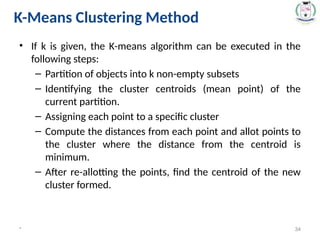
34. • If k is given, the K-means algorithm can be executed in the
following steps:
– Partition of objects into k non-empty subsets
– Identifying the cluster centroids (mean point) of the
current partition.
– Assigning each point to a specific cluster
– Compute the distances from each point and allot points to
the cluster where the distance from the centroid is
minimum.
– After re-allotting the points, find the centroid of the new
cluster formed.
* 34
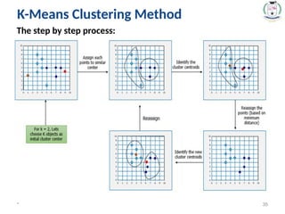
K-Means Clustering Method

35. The step by step process:
* 35
K-Means Clustering Method

36. * 36
K-Means Clustering Method

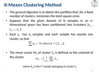
37. • The general objective is to obtain the partition that ,for a fixed
number of clusters, minimizes the total square error.
• Suppose that the given dataset of N samples in an n-
dimensional space has been partitioned into k-clusters {c1 ,
c2 ,... ck }.
• Each ck has nk samples and each sample has exactly one
cluster, so that
• The mean vector MK of cluster Ck is defined as the centroid of
the cluster
where Xik is the ith
sample belonging to cluster Ck
* 37
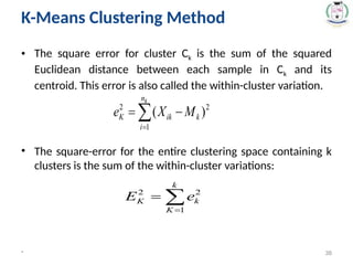
K-Means Clustering Method

38. • The square error for cluster Ck is the sum of the squared
Euclidean distance between each sample in Ck and its
centroid. This error is also called the within-cluster variation.
• The square-error for the entire clustering space containing k
clusters is the sum of the within-cluster variations:
* 38
K-Means Clustering Method

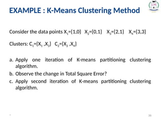
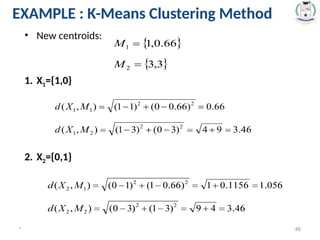
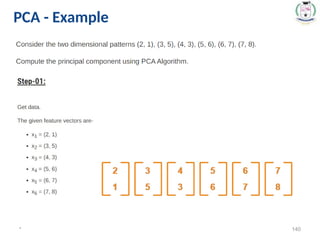
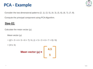
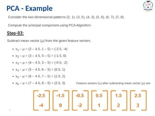
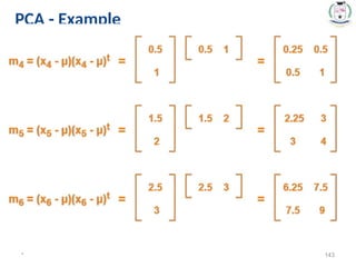
39. EXAMPLE : K-Means Clustering Method
Consider the data points X1={1,0} X2={0,1} X3={2,1} X4={3,3}
Clusters: C1={X1 ,X3} C2={X2 ,X4}
a. Apply one iteration of K-means partitioning clustering
algorithm.
b. Observe the change in Total Square Error?
c. Apply second iteration of K-means partitioning clustering
algorithm.
* 39
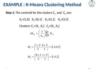
EXAMPLE : K-Means Clustering Method

40. Step 1: The centroid for the clusters C1 and C2 are:
* 40
X1={1,0} X2={0,1} X3={2,1} X4={3,3}
Clusters: C1={X1 ,X3} C2={X2 ,X4}
EXAMPLE : K-Means Clustering Method

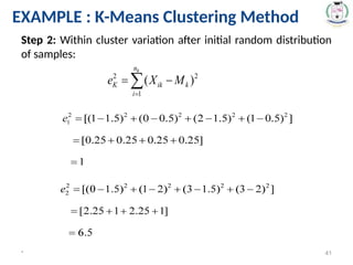
41. Step 2: Within cluster variation after initial random distribution
of samples:
* 41
EXAMPLE : K-Means Clustering Method

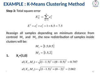
42. Step 3: Total square error
Reassign all samples depending on minimum distance from
centroid M1 and M2 ,the new redistribution of samples inside
clusters will be:
1. X1={1,0}
* 42
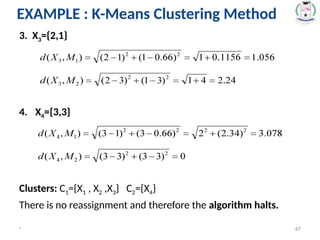
EXAMPLE : K-Means Clustering Method

43. 2. X2={0,1}
3. X3={2,1}
4. X4={3,3}
* 43
EXAMPLE : K-Means Clustering Method

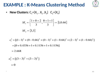
44. • New Clusters: C1={X1 , X2 ,X3} C2={X4}
* 44
EXAMPLE : K-Means Clustering Method

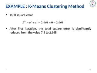
45. • Total square error
• After first iteration, the total square error is significantly
reduced from the value 7.5 to 2.668.
* 45
EXAMPLE : K-Means Clustering Method

46. • New centroids:
1. X1={1,0}
2. X2={0,1}
* 46
EXAMPLE : K-Means Clustering Method

47. 3. X3={2,1}
4. X4={3,3}
Clusters: C1={X1 , X2 ,X3} C2={X4}
There is no reassignment and therefore the algorithm halts.
* 47
EXAMPLE : K-Means Clustering Method

48. Advantages:
– With large number of variables, k-means may be
computationally faster that hierarchical clustering(if k is
small).
– K-means may produce tighter clusters that hierarchical
clustering especially is the cluster are globular.
Disadvantages:
– Difficult in comparing the quality of the clusters produced.
– Applicable only when mean is defined.
– Need to specify k, the number of clusters in advance.
– Unable to handle noisy data and outliers.
* 48
K-Means Clustering Method

49. DENSITY BASED CLUSTERING
* 49

50. DENSITY BASED CLUSTERING
• The density-based clustering method connects the highly-
dense areas into clusters, and the arbitrarily shaped
distributions are formed as long as the dense region can be
connected.
• This algorithm does it by identifying different clusters in the
dataset and connects the areas of high densities into clusters.
The dense areas in data space are divided from each other by
sparser areas.
• These algorithms can face difficulty in clustering the data
points if the dataset has varying densities and high
dimensions.
* 50
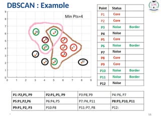
DBSCAN
OPTICS
DENCLUE
CLIQUE

51. * 51
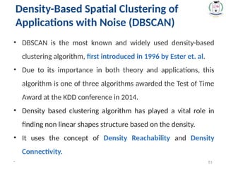
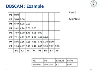
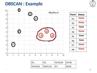
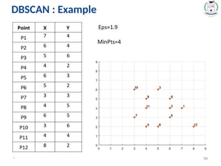
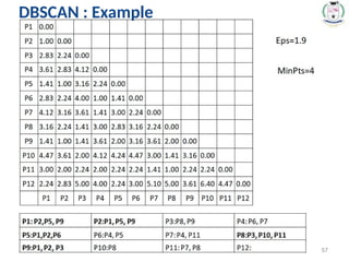
• DBSCAN is the most known and widely used density-based
clustering algorithm, first introduced in 1996 by Ester et. al.
• Due to its importance in both theory and applications, this
algorithm is one of three algorithms awarded the Test of Time
Award at the KDD conference in 2014.
• Density based clustering algorithm has played a vital role in
finding non linear shapes structure based on the density.
• It uses the concept of Density Reachability and Density
Connectivity.
Density-Based Spatial Clustering of
Applications with Noise (DBSCAN)

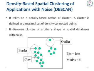
52. * 52
• It relies on a density-based notion of cluster: A cluster is
defined as a maximal set of density-connected points.
• It discovers clusters of arbitrary shape in spatial databases
with noise.
Density-Based Spatial Clustering of
Applications with Noise (DBSCAN)

53. * 53
DBSCAN : Example

54. * 54
DBSCAN : Example

55. * 55
DBSCAN : Example

56. * 56
DBSCAN : Example

57. * 57
DBSCAN : Example

58. * 58
DBSCAN : Example

59. * 59
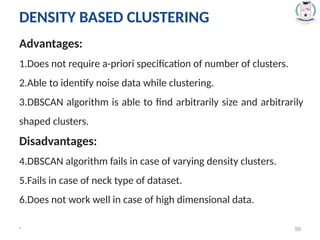
Advantages:
1.Does not require a-priori specification of number of clusters.
2.Able to identify noise data while clustering.
3.DBSCAN algorithm is able to find arbitrarily size and arbitrarily
shaped clusters.
Disadvantages:
4.DBSCAN algorithm fails in case of varying density clusters.
5.Fails in case of neck type of dataset.
6.Does not work well in case of high dimensional data.
DENSITY BASED CLUSTERING

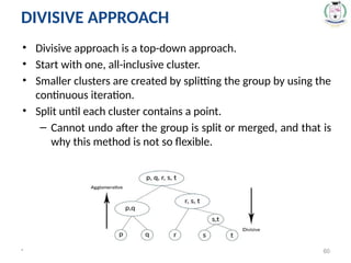
60. • Divisive approach is a top-down approach.
• Start with one, all-inclusive cluster.
• Smaller clusters are created by splitting the group by using the
continuous iteration.
• Split until each cluster contains a point.
– Cannot undo after the group is split or merged, and that is
why this method is not so flexible.
* 60
DIVISIVE APPROACH

61. * 61
Linkage Criterion: The linkage criterion is where exactly
the distance is measured.
Types of Linkage
⮚ Single-Linkage
⮚ Complete-Linkage
⮚ Average-Linkage
⮚ Centroid-Linkage
⮚ Ward’s Minimum Variance
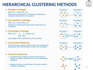
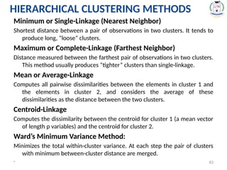
HIERARCHICAL CLUSTERING METHODS
HIERARCHICAL CLUSTERING METHODS

62. * 62
HIERARCHICAL CLUSTERING METHODS

63. * 63
Minimum or Single-Linkage (Nearest Neighbor)
Shortest distance between a pair of observations in two clusters. It tends to
produce long, “loose” clusters.
Maximum or Complete-Linkage (Farthest Neighbor)
Distance measured between the farthest pair of observations in two clusters.
This method usually produces “tighter” clusters than single-linkage.
Mean or Average-Linkage
Computes all pairwise dissimilarities between the elements in cluster 1 and
the elements in cluster 2, and considers the average of these
dissimilarities as the distance between the two clusters.
Centroid-Linkage
Computes the dissimilarity between the centroid for cluster 1 (a mean vector
of length p variables) and the centroid for cluster 2.
Ward’s Minimum Variance Method:
Minimizes the total within-cluster variance. At each step the pair of clusters
with minimum between-cluster distance are merged.
HIERARCHICAL CLUSTERING METHODS

64. * 64
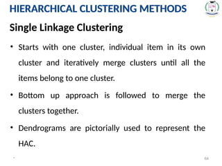
HIERARCHICAL CLUSTERING METHODS
• Starts with one cluster, individual item in its own
cluster and iteratively merge clusters until all the
items belong to one cluster.
• Bottom up approach is followed to merge the
clusters together.
• Dendrograms are pictorially used to represent the
HAC.
Single Linkage Clustering
HIERARCHICAL CLUSTERING METHODS

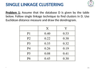
65. Problem 1: Assume that the database D is given by the table
below. Follow single linkage technique to find clusters in D. Use
Euclidean distance measure and draw the dendrogram.
* 65
SINGLE LINKAGE CLUSTERING

66. Solution:
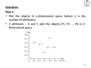
Step 1:
• Plot the objects in n-dimensional space (where n is the
number of attributes).
• 2 attributes – X and Y, plot the objects P1, P2, … P6 in 2-
dimensional space:
* 66

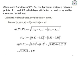
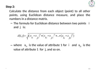
67. Step 2:
Calculate the distance from each object (point) to all other
points, using Euclidean distance measure, and place the
numbers in a distance matrix.
– The formula for Euclidean distance between two points i
and j is:
– where xi1 is the value of attribute 1 for i and xj1 is the
value of attribute 1 for j, and so on.
* 67

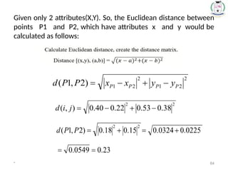
68. Given only 2 attributes(X,Y). So, the Euclidean distance between
points P1 and P2, which have attributes x and y would be
calculated as follows:
* 68

69. * SIT1305 Machine 69
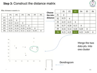
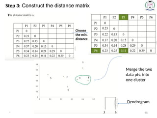
Choose
the min.
distance
Merge the two
data pts. into
one cluster
Dendrogram
Step 3: Construct the distance matrix

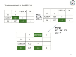
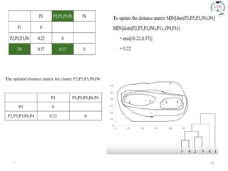
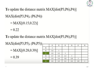
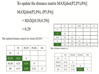
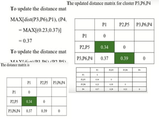
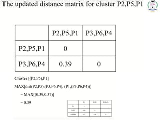
70. * 70
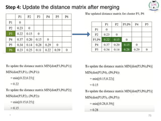
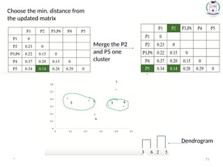
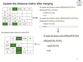
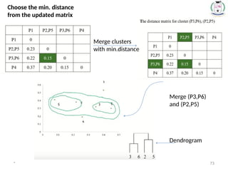
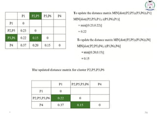
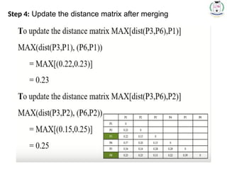
Step 4: Update the distance matrix after merging

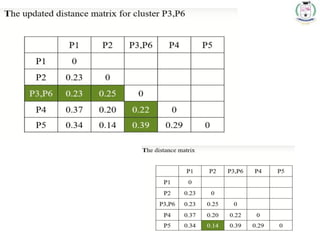
71. * 71
Choose the min. distance from
the updated matrix
Merge the P2
and P5 one
cluster
Dendrogram

72. * 72
Update the distance matrix after merging

73. * 73
Choose the min. distance
from the updated matrix
Merge clusters
with min.distance
Merge (P3,P6)
and (P2,P5)
Dendrogram

74. * 74

75. * 75
Choose
the min.
distance
Merge
(P3,P6,P2,P5)
and P4

76. * 76
Dendrogram

77. * 77

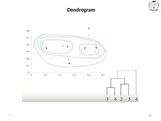
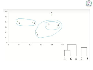
78. * 78
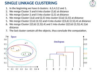
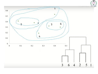
1. In the beginning we have 6 clusters : 6,5,4,3,2 and 1.
2. We merge Cluster 3 and 6 into cluster (3,6) at distance
3. We merge Cluster 2 and 5 into cluster (2,5) at distance
4. We merge Cluster (3,6) and (2,5) into cluster ((3,6) (2,5)) at distance
5. We merge Cluster ((3,6) (2,5)) and 4 into cluster (((3,6) (2,5)),4) at distance
6. We merge Cluster (((3,6) (2,5)),4) and 1 into cluster ((((3,6) (2,5)),4),1)at
distance
7. The last cluster contain all the objects, thus conclude the computation.
SINGLE LINKAGE CLUSTERING

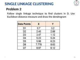
79. * 79
Problem 2
Follow single linkage technique to find clusters in D. Use
Euclidean distance measure and draw the dendrogram
SINGLE LINKAGE CLUSTERING

80. * 80
HIERARCHICAL CLUSTERING METHODS
• Starts with one cluster, individual item in its own
cluster and iteratively merge clusters until all the
items belong to one cluster.
• Bottom up approach is followed to merge the
clusters together.
• Dendrograms are pictorially used to represent the
HAC.
Complete Linkage Clustering

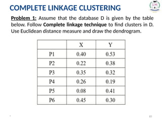
81. Problem 1: Assume that the database D is given by the table
below. Follow Complete linkage technique to find clusters in D.
Use Euclidean distance measure and draw the dendrogram.
* 81
COMPLETE LINKAGE CLUSTERING

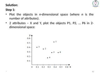
82. Solution:
Step 1:
• Plot the objects in n-dimensional space (where n is the
number of attributes).
• 2 attributes – X and Y, plot the objects P1, P2, … P6 in 2-
dimensional space:
* 82

83. Step 2:
Calculate the distance from each object (point) to all other
points, using Euclidean distance measure, and place the
numbers in a distance matrix.
– The formula for Euclidean distance between two points i
and j is:
– where xi1 is the value of attribute 1 for i and xj1 is the
value of attribute 1 for j, and so on.
* 83

84. Given only 2 attributes(X,Y). So, the Euclidean distance between
points P1 and P2, which have attributes x and y would be
calculated as follows:
* 84

85. * 85
Choose
the min.
distance
Merge the two
data pts. into
one cluster
Dendrogram
Step 3: Construct the distance matrix

86. Step 4: Update the distance matrix after merging

87. * 87

96. * 96
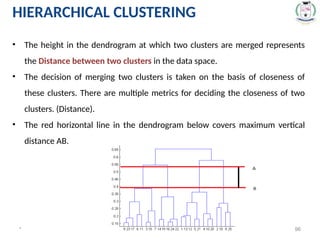
• The height in the dendrogram at which two clusters are merged represents
the Distance between two clusters in the data space.
• The decision of merging two clusters is taken on the basis of closeness of
these clusters. There are multiple metrics for deciding the closeness of two
clusters. (Distance).
• The red horizontal line in the dendrogram below covers maximum vertical
distance AB.
HIERARCHICAL CLUSTERING

97. * 97
Advantages:
•We can obtain the optimal (desired) number of clusters from
the model itself, human intervention not required.
•Dendrograms help us in clear visualization, which is practical
and easy to understand.
Disadvantages:
•Not suitable for large datasets due to high time and space
complexity.
•In hierarchical Clustering, once a decision is made to combine
two clusters, it can not be undone.
•The time complexity for the clustering can result in very
long computation times.
HIERARCHICAL CLUSTERING

98. a. Search Engine Result Grouping.
b. Document Clustering.
c. Banking and Insurance fraud detection.
d. Image Segmentation.
e. Customer Segmentation.
f. Recommendation Engines.
g. Social Network Analysis.
h. Network Traffic Analysis.
* 98
APPLICATIONS OF CLUSTERING

99. CLUSTERING METHODS
* 99

100. * 100
CLUSTERING METHODS

101. GRID BASED CLUSTERING METHODS
* 101

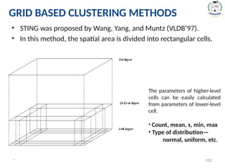
102. • STING was proposed by Wang, Yang, and Muntz (VLDB’97).
• In this method, the spatial area is divided into rectangular cells.
* 102
The parameters of higher-level
cells can be easily calculated
from parameters of lower-level
cell.
• Count, mean, s, min, max
• Type of distribution—
normal, uniform, etc.
GRID BASED CLUSTERING METHODS

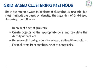
103. There are multiple ways to implement clustering using a grid, but
most methods are based on density. The algorithm of Grid-based
clustering is as follows −
– Represent a set of grid cells.
– Create objects to the appropriate cells and calculate the
density of each cell.
– Remove cells having a density below a defined threshold, r.
– Form clusters from contiguous set of dense cells.
* 103
GRID BASED CLUSTERING METHODS

104. * 104
• The grid-based clustering methods use a multi-resolution grid data
structure.
• It quantizes the object areas into a finite number of cells that form a grid
structure on which all of the operations for clustering are implemented.
The benefit of the method is its quick processing time, which is generally
independent of the number of data objects, still dependent on only the
multiple cells in each dimension in the quantized space.
• An instance of the grid-based approach involves STING, which explores
statistical data stored in the grid cells.
• WaveCluster, which clusters objects using a wavelet transform approach,
and CLIQUE, which defines a grid-and density-based approach for
clustering in high-dimensional data space
GRID BASED CLUSTERING METHODS

105. * 105
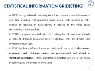
• A STING is a grid-based clustering technique. It uses a multidimensional
grid data structure that quantifies space into a finite number of cells.
Instead of focusing on data points, it focuses on the value space
surrounding the data points.
• In STING, the spatial area is divided into rectangular cells and several levels
of cells at different resolution levels. High-level cells are divided into
several low-level cells.
• In STING Statistical Information about attributes in each cell, such as mean,
maximum, and minimum values, are precomputed and stored as
statistical parameters. These statistical parameters are useful for query
processing and other data analysis tasks
STATISTICAL INFORMATION GRID(STING)

106. * 106
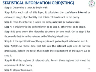
Step 1: Determine a layer, to begin with.
Step 2: For each cell of this layer, it calculates the confidence interval or
estimated range of probability that this is cell is relevant to the query.
Step 3: From the interval, it labels the cell as relevant or not relevant.
Step 4: If this layer is the bottom layer, go to step 6, otherwise, go to step 5.
Step 5: It goes down the hierarchy structure by one level. Go to step 2 for
those cells that form the relevant cell of the high-level layer.
Step 6: If the specification of the query is met, go to step 8, otherwise step 7.
Step 7: Retrieve those data that fall into the relevant cells and do further
processing. Return the result that meets the requirement of the query. Go to
step 9.
Step 8: Find the regions of relevant cells. Return those regions that meet the
requirement of the query.
Step 9: Stop or terminate.
STATISTICAL INFORMATION GRID(STING)

107. * 107
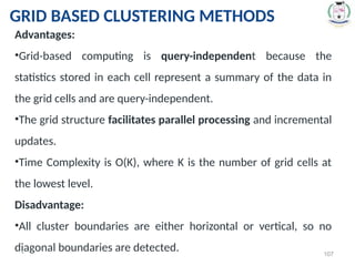
Advantages:
•Grid-based computing is query-independent because the
statistics stored in each cell represent a summary of the data in
the grid cells and are query-independent.
•The grid structure facilitates parallel processing and incremental
updates.
•Time Complexity is O(K), where K is the number of grid cells at
the lowest level.
Disadvantage:
•All cluster boundaries are either horizontal or vertical, so no
diagonal boundaries are detected.
GRID BASED CLUSTERING METHODS

108. DIMENSIONALITY REDUCTION

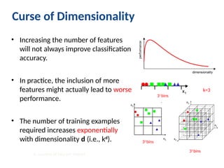
109. Curse of Dimensionality
• Increasing the number of features
will not always improve classification
accuracy.
• In practice, the inclusion of more
features might actually lead to worse
performance.
• The number of training examples
required increases exponentially
with dimensionality d (i.e., kd
). 32
bins
33
bins
31
bins
k: number of bins per feature
k=3

110. 110
Dimensionality Reduction
• What is the objective?
– Choose an optimum set of features of lower
dimensionality to improve classification accuracy.
• Different methods can be used to reduce
dimensionality:
– Feature extraction
– Feature selection

111. 111
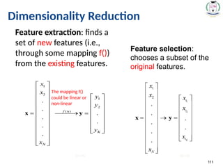
Dimensionality Reduction
Feature extraction: finds a
set of new features (i.e.,
through some mapping f())
from the existing features.
Feature selection:
chooses a subset of the
original features.
The mapping f()
could be linear or
non-linear
K<<N K<<N

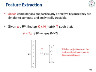
112. Feature Extraction
• Linear combinations are particularly attractive because they are
simpler to compute and analytically tractable.
• Given x R
ϵ N
, find an K x N matrix T such that:
y = Tx R
ϵ K
where K<<N
112
T This is a projection from the
N-dimensional space to a K-
dimensional space.

113. • From a mathematical point of view, finding an optimum
mapping y= (
𝑓 x) is equivalent to optimizing an objective
criterion.
• Different methods use different objective criteria, e.g.,
– Minimize Information Loss: represent the data as accurately as possible
in the lower-dimensional space.
– Maximize Discriminatory Information: enhance the class-discriminatory
information in the lower-dimensional space.
113
Feature Extraction

114. • Popular linear feature extraction methods:
– Principal Components Analysis (PCA): Seeks a projection that
preserves as much information in the data as possible.
– Linear Discriminant Analysis (LDA): Seeks a projection that best
discriminates the data.
• Many other methods:
– Making features as independent as possible (Independent Component
Analysis or ICA).
– Retaining interesting directions (Projection Pursuit).
– Embedding to lower dimensional manifolds (Isomap, Locally Linear
Embedding or LLE).
114
Feature Extraction

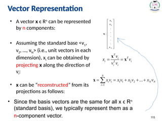
115. Vector Representation
• A vector x ϵ Rn
can be represented
by n components:
• Assuming the standard base <v1,
v2, …, vN> (i.e., unit vectors in each
dimension), xi can be obtained by
projecting x along the direction of
vi:
• x can be “reconstructed” from its
projections as follows:
115
• Since the basis vectors are the same for all x R
ϵ n
(standard basis), we typically represent them as a
n-component vector.
Vector Representation

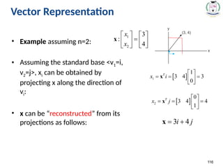
116. • Example assuming n=2:
• Assuming the standard base <v1=i,
v2=j>, xi can be obtained by
projecting x along the direction of
vi:
• x can be “reconstructed” from its
projections as follows:
116
i
j
Vector Representation

117. LINEAR DISCRIMINANT ANALYSIS
* 117

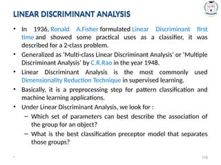
118. • In 1936, Ronald A.Fisher formulated Linear Discriminant first
time and showed some practical uses as a classifier, it was
described for a 2-class problem.
• Generalized as ‘Multi-class Linear Discriminant Analysis’ or ‘Multiple
Discriminant Analysis’ by C.R.Rao in the year 1948.
• Linear Discriminant Analysis is the most commonly used
Dimensionality Reduction Technique in supervised learning.
• Basically, it is a preprocessing step for pattern classification and
machine learning applications.
• Under Linear Discriminant Analysis, we look for :
– Which set of parameters can best describe the association of
the group for an object?
– What is the best classification preceptor model that separates
those groups?
* 118
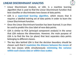
LINEAR DISCRIMINANT ANALYSIS
LINEAR DISCRIMINANT ANALYSIS

119. • Linear Discriminant Analysis, or LDA, is a machine learning
algorithm that is used to find the Linear Discriminant function that
best classifies or discriminates two classes of data points.
• LDA is a supervised learning algorithm, which means that it
requires a labelled training set of data points in order to learn the
Linear Discriminant function.
• Once the Linear Discriminant function has been learned, it can then
be used to predict the class label of new data points.
• LDA is similar to PCA (principal component analysis) in the sense
that LDA reduces the dimensions. However, the main purpose of
LDA is to find the line (or plane) that best separates data points
belonging to different classes.
• The key idea behind LDA is that the decision boundary should be
chosen such that it maximizes the distance between the means of
the two classes while simultaneously minimizing the variance
within each classes data or within-class scatter.
* 119
LINEAR DISCRIMINANT ANALYSIS

120. * 120
LINEAR DISCRIMINANT ANALYSIS- MODEL

121. * 121
LINEAR DISCRIMINANT ANALYSIS
Distributing variables into two or more classes.

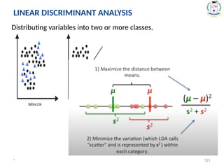
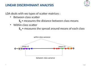
122. * 122
LDA deals with wo types of scatter matrices :
• Between class scatter
Sb = measures the distance between class means
• Within class scatter
Sw = measures the spread around means of each class
LINEAR DISCRIMINANT ANALYSIS

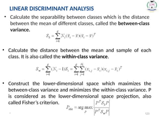
123. * 123
• Calculate the separability between classes which is the distance
between the mean of different classes, called the between-class
variance.
LINEAR DISCRIMINANT ANALYSIS
• Calculate the distance between the mean and sample of each
class. It is also called the within-class variance.
• Construct the lower-dimensional space which maximizes the
between-class variance and minimizes the within-class variance. P
is considered as the lower-dimensional space projection, also
called Fisher’s criterion.

124. * 124
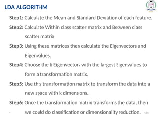
Step1: Calculate the Mean and Standard Deviation of each feature.
Step2: Calculate Within class scatter matrix and Between class
scatter matrix.
Step3: Using these matrices then calculate the Eigenvectors and
Eigenvalues.
Step4: Choose the k Eigenvectors with the largest Eigenvalues to
form a transformation matrix.
Step5: Use this transformation matrix to transform the data into a
new space with k dimensions.
Step6: Once the transformation matrix transforms the data, then
we could do classification or dimensionality reduction.
LDA ALGORITHM

125. * 125
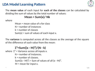
LDA Model Learning Pattern
The mean value of each input for each of the classes can be calculated by
dividing the sum of values by the total number of values:
Mean = Sum(x)/ Nk
where
Mean = mean value of x for class
N = number of instances
k = number of classes
Sum(x) = sum of values of each input x.
The variance is computed across all the classes as the average of the square
of the difference of each value from the mean:
Σ²=Sum((x - M)²)/(N - k)
where Σ² = Variance across all inputs x.
N = number of instances.
k = number of classes.
Sum((x - M)²) = Sum of values of all (x - M)².
M = mean for input x.

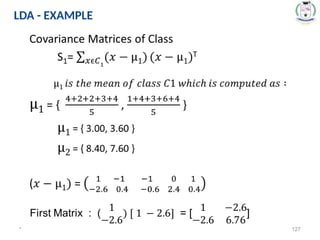
126. Goal : To project a feature space (N-Dimensional Data)
on to a smaller subspace k (k<= N-1) while maintaining
the class discriminating information.
Consider a 2-D Data set
C1=(x1,y1) = { (4,1) (2,4) (2,3) (3,6) (4,4) }
C2=(x2,y2) = { (9,10) (6,8) (9,5) (8,7) (10,8) }
Step1: Compute within_class Scatter Matrix Sw
Sw = S1 + S2
S1 is the Covariance Matrix for the class C1 and S2 is the
Covariance Matrix for the class C2
* 126
LDA - EXAMPLE

127. * 127
LDA - EXAMPLE

128. * 128
•
LDA - EXAMPLE

129. * 129
LDA - EXAMPLE

130. •
* 130
LDA - EXAMPLE

131. * 131
LDA - EXAMPLE

132. •
* 132
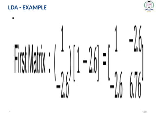
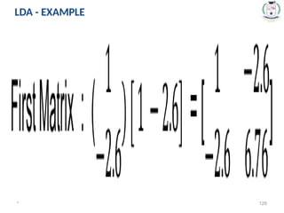
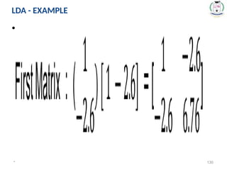
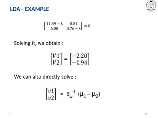
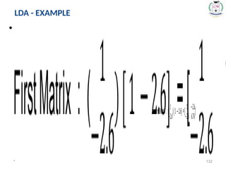
LDA - EXAMPLE

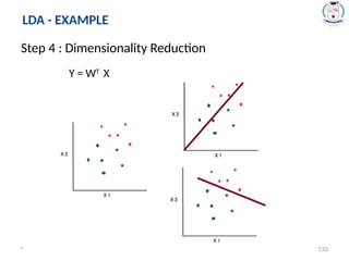
133. * 133
Step 4 : Dimensionality Reduction
Y = WT
X
LDA - EXAMPLE

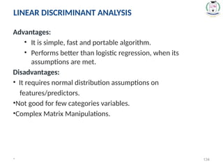
134. Advantages:
• It is simple, fast and portable algorithm.
• Performs better than logistic regression, when its
assumptions are met.
Disadvantages:
• It requires normal distribution assumptions on
features/predictors.
•Not good for few categories variables.
•Complex Matrix Manipulations.
* 134
LINEAR DISCRIMINANT ANALYSIS

135. PRINCIPLE COMPONENT ANALYSIS
* 135

136. * 136
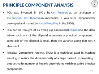
PRINCIPLE COMPONENT ANALYSIS
• PCA was invented in 1901 by Karl Pearson, as an analogue of
the principal axis theorem in mechanics, it was later independently
developed and named by Harold Hotelling in the 1930s.
• PCA can be thought of as fitting a p-dimensional ellipsoid to the data,
where each axis of the ellipsoid represents a principal component. If
some axis of the ellipsoid is small, then the variance along that axis is
also small.
• Principal Component Analysis (PCA) is a technique used in machine
learning to reduce the dimensionality of a large dataset by projecting it
onto a smaller number of linearly uncorrelated variables called principal
components.

137. * 137
PRINCIPLE COMPONENT ANALYSIS

138. * 138
PCA - ALGORITHM
Step 1 - Load data : Let's say we have a dataset with n data points,
where each data point has m features. We load the data into a matrix X
of size n x m.
Step 2 - Center data : center the data by subtracting the mean of each
feature from each data point. This ensures that each feature has a
mean of zero.
Step 3 - Compute covariance matrix : compute the covariance matrix of
the centered data, which is a measure of how much two features vary
together. The covariance matrix is a square matrix of size m x m.
Step 4 - Compute eigenvectors and eigenvalues of covariance matrix :
compute the eigenvectors and eigenvalues of the covariance matrix.
The eigenvectors are a set of orthogonal vectors that define the
directions of the principal components, and the eigenvalues represent
the variance of the data along these directions.

139. * 139
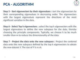
Step 5 - Sort eigenvectors by their eigenvalues : sort the eigenvectors by
their corresponding eigenvalues in decreasing order. The eigenvectors
with the largest eigenvalues represent the directions of the most
significant variation in the data.
Step 6 - Select Top k eigenvectors : select the top k eigenvectors with the
largest eigenvalues to define the new subspace for the data, thereby
choosing the principle components. Typically, we choose k to be much
smaller than m to reduce the dimensionality of the data.
Step 7 - Project the data onto the new subspace : Project the centered
data onto the new subspace defined by the top k eigenvectors to obtain
the new dataset Y. The size of Y is n x k.
PCA - ALGORITHM

140. * 140
PCA - Example

141. * 141
PCA - Example

142. * 142
PCA - Example

143. * 143
PCA - Example

144. * 144
PCA - Example

145. * 145
PCA - Example

146. * 146
PCA - Example
Step-06:

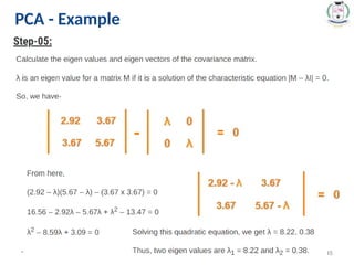
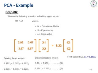
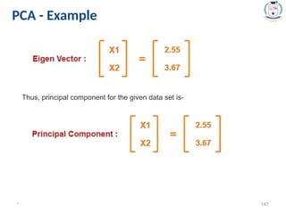
147. * 147
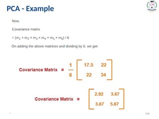
PCA - Example
Thus, principal component for the given data set is-

148. * 148
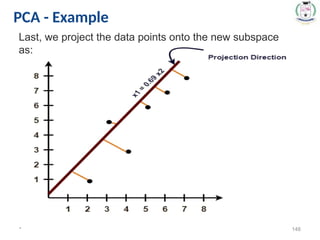
PCA - Example
Last, we project the data points onto the new subspace
as:

149. Advantages:
• Removes correlated features.
• Improves machine learning algorithm performance.
• Reduce overfitting.
Disadvantages:
•Independent variables are now less interpretable.
•Information loss.
•Feature scaling
* 149
PRINCIPLE COMPONENT ANALYSIS