Downloaded 19 times


![Measuring the Dispersion of Data
Quartiles, outliers and boxplots
» Quartiles: Q1 (25th percentile), Q3 (75th percentile)
» Inter-quartile range: IQR = Q3 – Q1
» Five number summary: min, Q1, M, Q3, max
» Boxplot: ends of the box are the quartiles, median is marked,
whiskers, and plot outlier individually
» Outlier: usually, a value higher/lower than 1.5 x IQR
Variance and standard deviation
» Variance s2: (algebraic, scalable computation)
» Standard deviation s is the square root of variance s2
s
2
=
1
n − 1
n
∑
i=1
(x
i
− x )
2
=
n
1
[∑ x
n − 1 i=1
2
i
−
n
1
(∑ xi)
n
i=1
2
]
39
Boxplot Analysis
Five-number summary of a distribution:
Minimum, Q1, M, Q3, Maximum
Boxplot
» Data is represented with a box
» The ends of the box are at the first and
third quartiles, i.e., the height of the box is
IRQ
» The median is marked by a line within the
box
» Whiskers: two lines outside the box extend
to Minimum and Maximum
40](https://image.slidesharecdn.com/characterization-131222082300-phpapp02/85/Characterization-20-320.jpg)


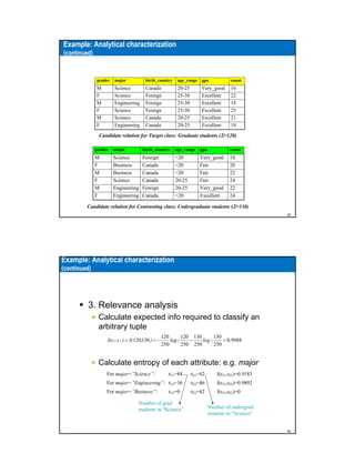
The document discusses characterization in data mining. It covers concept description through data generalization and summarization to provide characterization. Analytical characterization involves analyzing attribute relevance. Mining class comparisons allows discriminating between different classes by comparing generalized descriptions. Descriptive statistical measures can also be mined from large databases to characterize data dispersion through measures of central tendency, variation, and outliers.