This document discusses aquifer testing, which involves pumping a well and measuring the water level response over time. This allows evaluation of the well and aquifer properties, including productivity, efficiency and hydraulic characteristics. A typical test involves constant pumping for 1-30 days while measuring water level changes. Test results indicate aquifer transmissivity and storage, and whether the aquifer can support the intended water demand. Factors like test duration, measurement accuracy, and avoiding interference, are important for properly analyzing results and understanding the aquifer boundaries and properties.

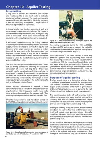
1. 88
Introduction
A key area of interest for individual well owners
and regulators alike is how much water a particular
aquifer or well can produce. The most common and
dependable way of establishing this is by pumping
a well and measuring its response. This procedure is
known as a pump test or aquifer test.
A typical aquifer test involves pumping a well at a
constant rate for a certain period of time. The change in
aquifer level at the pumped well, and in neighbouring
wells is measured. From these measurements the
aquifer or well hydraulic properties can be evaluated.
It will usually be obvious during the drilling process if
a well will provide the volumes required for a domestic
supply, without the need to carry out an aquifer test.
However where larger volumes are required at certain
times of the year, such as for frost protection, crop
irrigation or town supply, it may not be as clear-cut.
In this case detailed seasonal test information may be
needed to select the most efficient pump type and to
prove reliable flows exist.
The most frequently conducted tests are those carried
out by drilling contractors following the successful
completion of a new well (Fig. 10.1). These tests
generally involve pumping the well for several hours to
test the well’s capacity. The test results can also be used
to assess the value of the aquifer hydraulic properties
of transmissivity and storativity. Knowledge of these
wider aquifer parameters allows the performance of a
well to be forecast into the future.
Where detailed information is needed, a more
comprehensive test is carried out. These tests can last
anywhere from 1 to 30 days and involve many wells,
some at large distances from the pumped well. They
normally involve pumping the well at a constant rate.
Over the years, numerous tests have been carried out
by the MDC or its predecessors, and private well owners
for a variety of purposes. During the 1980s and 1990s,
the focus of MDC testing was to measure the hydraulic
properties of lesser understood aquifers, mostly in the
Southern Valleys Catchments (Fig. 10.2).
Historically the MDC has been involved in some way
either in a general role, by providing water level or
flow measuring equipment, but this is less common in
recent times. With the expansion of irrigated vineyard
into areas where there are competing demands for
groundwater, aquifer testing is increasingly required to
quantify interference effects between wells. These are
commissioned by private concerns and supervised by
consultants rather than regulators.
Purpose of aquifer testing
The key aim of a test is to determine whether there
is sufficient groundwater available for the proposed
use. The most important information that is collected
as part of an aquifer test is the depth to groundwater
and how that varies in response to pumping the well
of interest, and how well water levels vary seasonally.
The most important index of well behaviour is the
difference between the water level at rest and the
pumping level, which is called the drawdown. Larger
drawdowns are associated with higher pumping rates
or lower producing wells or aquifers (Fig. 10.3).
The higher yielding an aquifer or well, the smaller the
drawdown for a given flow rate and the faster water
levels will recover once pumping stops. Generally
drawdown increases the longer pumping continues
and is greatest in the pumped well and reduces with
distance (Fig. 10.4).
For an individual well owner, testing the productivity
or efficiency of their well will be of prime importance.
For MDC the wider characteristics of how transmissive
it is and how much groundwater it stores, would be
the focus for regional scale water management. The
storage of an aquifer can only be calculated if there
Figure 10.1: A very large surface mounted pump being used to
test the Bar test well (1733) during a 72 hour test in 1987
Figure 10.2: Peter Davidson manually dipping the depth to the
water table during a pump test - 1987
Chapter 10 - Aquifer Testing

2. 89
are measurements of the change in water level at
observation wells. In other words there must be
measurements in three dimensions over time to
calculate a volumetric change in groundwater stored
in an aquifer. Sometimes the information provided
by pumping a single well will be all that is required,
providing information such as aquifer transmissivity,
well capacity and efficiency.
No two aquifer tests are the same because of the
uniqueness of aquifer properties and individual
well circumstances. Generally tests in unconfined
aquifers last longer than those performed on wells
tapping confined aquifers. This reflects the naturally
higher storage properties associated with unconfined
aquifers, meaning that the effects of the pumping are
spread more slowly over space and time. This delay is
an important consideration if interference effects are
being assessed.
The minimum duration of a test for an unconfined
aquifer is usually three days, compared to one day for
the same flow rate in a confined aquifer. The aim of the
test will also have a major bearing on the test duration
and must be looked at on a case by case basis.
Tests can be broadly split into those using a constant
flowrate, and those with a pumping rate that varies
over time. Step drawdown tests are a common type
of variable flow test which involve pumping a well at
a variety of rates over a short period for the purpose
of measuring its yield and efficiency (Fig. 10.5). The
analysis of this information allows the behaviour of
the well to be mathematically described and provides
a very useful way of forecasting its performance
under different operating scenarios based on the well
efficiency.
Constant discharge tests provide information about
the interaction of a well with its neighbour, and just
as importantly the nature of any aquifer boundaries.
A commonly asked question is whether an aquifer is
large or small or does a particular well interact with a
nearby spring or river? The nature of the test results
plotted in a standard manner can identify what are
known as boundary effects with each type having a
distinctive signature.
Figure 10.4: Aquifer test layout
Figure 10.3: Definition of well terms
0 100 200 300 400 500 600 700
-20
-15
-10
-5
0
Drawdown(Metres)
Time (Minutes)
Figure 10.5: Step drawdown test procedure for well 0864
tapping the Benmorven Aquifer during the late 1980s. Each step
represents a different flow rate

3. 90
Largeaquifershavemorestoragethansmallerones,and
as a consequence the cone of depression developed
when a well is pumped, is unlikely to expand radially
outwards sufficiently far to intercept a boundary.
However if a well tapping a geographically small or low
yielding aquifer bounded by basement rock is pumped
at a high enough rate, the drawdown will steepen
over time. This indicates the cone of depression has
intercepted the edge of the aquifer.
Aquifer response to pumping
Wells respond in characteristic ways to pumping,
which tell a story about their hydraulic properties and
boundaries.
A feature of the drawdown generated by aquifer tests
is the symmetry between the well or aquifer response
during the initial drawdown phase caused by the pump
starting, compared to the later recovery phase when
the pump stops (Fig. 10.6).
During a 1998 constant drawdown test carried out
on well 3291 penetrating the Deep Wairau Aquifer,
pumping occurred at a rate of 3,100 m3
/day for three
days (Fig. 10.6). The static or non-pumping pressure at
well 3291 was measured to be 12.7 metres above the
well-head prior to the test using a long clear hose and
a cherry picker. This was almost as high as the nearby
power lines.
A special type of drawdown response occurs within
unconfined aquifers involving gravity drainage of
groundwater (Fig. 10.7). During the first ten minutes
of the unconfined aquifer test, the drawdown is similar
to that of a confined aquifer with groundwater mainly
being sourced by horizontal flow. During the middle
part of the test the rate of drawdown starts to level off.
This response is known as delayed yield and is caused
by the vertical drainage of water stored in the overlying
sand. In the later part of the test, after about an hour,
this storage is used up and the curve starts to follow
the response of a confined aquifer again.
Aquifer boundaries
Distortions to the cone of depression occur when an
aquifer boundary is encountered. There are two main
types of boundary, an impermeable boundary such
as bedrock and a recharge boundary such as a stream
(Fig. 10.8). A steady flow allows the effects of aquifer
boundaries to be identified.
An example, the 1998 pump test of well 3278 showed
twochangesofslopeat900and1800minutes,indicating
the presence of several impermeable barriers nearby
(Fig. 10.9). With a knowledge of aquifer storage it is
possible to estimate the distance to these boundaries
based on the travel time of the cone of depression and
the time since pumping started. The time the cone of
depression has taken to expand outwards to intercept
this well coincides with the fall in well level at around
250 minutes, in which time it has travelled a distance
of 1,600 metres. Water levels did not rebound to their
original level after pumping stopped at 4,000 minutes.
Instead of groundwater levels bouncing back, they have
remained subdued. This indicates a low storage aquifer
with more water being pumped out than is naturally
replacing it and is consistent with the presence of
boundaries and an aquifer of limited extent.
0.01
0.10
1 10 100 1,000
Time (minutes)
Drawdown(m)
Observed Data
Boulton Prediction
0
10
20
30
40
50
0 1000 2000 3000 4000 5000
ELAPSED TIME (minutes)
DRAWDOWN(metres)
Figure 10.6: Constant discharge test well response for confined
aquifer well 3291 tapping the Deep Wairau Aquifer in 1998
Figure 10.7: Constant discharge test well response for
unconfined Rarangi Shallow Aquifer
Figure 10.8: Aquifer boundary types

4. 91
Some natural effects such as ocean tides are always
present at coastal wells and can’t be avoided, but can
be allowed for. The measurements from longer term
testsnormallyrequirecorrectionasnaturalbackground
changes in aquifer status either through drainage or
recharge have a significant influence after several days.
Accurate measurement of test flows and the resulting
changes in groundwater level, are essential for correctly
evaluating aquifer and well hydraulic properties. In the
past the depth to the water table was measured using an
oversized tape measure which consisted of a calibrated
tape with a weight on the end (Fig. 10.11). When the
water table was reached, a circuit was completed and a
light or buzzer went on at the surface. Automatic water
level recorders are now more commonly used as they
can take more frequent measurements, including the
leadup and recovery phases.
The opposite occurs in an aquifer that is leaky or
connected to a recharge source such as a nearby
stream, as the drawdown curve will flatten over time
as more groundwater is drawn into the aquifer in
response to pumping (Fig. 10.10). In other words, the
fall in groundwater levels is lessened.
Test methods and procedures
There are many practical difficulties to contend with
when it comes to aquifer testing under Marlborough
conditions. Most revolve around having stable
environmental conditions so there is no external
interference to the test. It is important to avoid
recharge events such as heavy rain or river floods, or
the influence of other pumping which can disturb
drawdown measurements.
Figure 10.9: Multiple barrier boundaries at well 3278 located
1600 metres north-west of the pumped well.
Figure 10.11: Manually measuring groundwater level in a shallow
well (1856) at Benmorven in 1990
Figure 10.10: Drawdown test conducted on the Huia well 4402 in
the Riverlands Aquifer
Figure 10.13: Bar test well flow measurement. Three orifice
flow meters were required to measure the large flows
involved with the testing of the MCRWB Bar test well (1733)
tapping the high yielding coastal Wairau Aquifer in 1987.
0
500
1000
1500
1 10 100 1000 10000
Time (minutes)
Drawdown(millimetres)
boundary1
boundary2
5.0
5.5
6.0
6.5
7.0
7.5
8.0
8.5
9.0
1 10 100 1,000
Time (minutes)
Drawdown(m)
Theis Prediction
Boulton Prediction
Observed Data
Figure 10.12: Temporary standpipe erected to measure the
artesian pressures during the Benmorven Aquifer test in
December 1990. The observer had to climb up the ladder and
read the level of groundwater sitting in a clear plastic tube
attached to the pole. This wasn’t as easy as it sounds at night.

5. 92
Due to the presence of artesian groundwater levels
during some tests, stand pipes consisting of clear
plastic tubes are sometimes used to measure their
elevation (Fig. 10.12).
Orifice flow meters have been the most common
method of measuring test flow rates, although
electronic meters are becoming more prevalent.
Orifice meters work on the principle that the flow of
water through a hole of a given size is proportional to
the pressure in the vessel and measured in stand pipes
(Fig. 10. 13 and Fig. 10.14).
Another consideration is the recirculation of discharged
groundwater back into the aquifer. This is a particular
Figure 10.15: Discharged test water being piped north along Mill
Road at Wairau Valley to Mill Stream during the December 2006
MDC test.
Figure 10.16: Test discharge water being disposed of at
RNZAF Base Woodbourne in the early 1980s. A lined trench
has been excavated to allow water to be directed away
without infiltrating back to groundwater.
problem in free draining, unconfined
aquifers where water will rapidly return
to the water table and cause drawdown
measurements to be smaller than would
otherwise be the case. To overcome
this, water is piped well away from the
measurement wells to avoid affecting
them, often to a stream which has a
sealed bed (Fig. 10.15 and Fig. 10.16).
One of the major differences in the test
response of wells tapping high versus
low yielding aquifers is the degree to
which equilibrium conditions develop
with time. When measurements show
the water table remains at a constant
depth over time this shows a balance
exists between the rate groundwater is
being pumped from the well versus the
rate of aquifer recharge. This is referred
to as steady state conditions and is
commonly associated with high yielding
or leaky type aquifers, and also where a
stream is a major source of recharge.
Unsteady conditions reflect a falling well water table
over time due to more water being removed from the
aquifer than is being naturally replaced. This is the
normal situation in low yielding aquifers such as those
underlying the Southern Valleys catchments.
Unchanging or steady state conditions make it difficult
to meaningfully interpret the value of aquifer hydraulic
properties because they are masked by boundary
influences. High yielding wells or aquifers require
higher test pump rates than low yielding aquifers to
generate sufficient drawdown to calculate aquifer
properties. In turn this determines the pump size
and affects how the test water is disposed of. All are
important practical considerations.
Figure 10.14: A single flow meter was sufficient for the small test rate used to
evaluate the very low yielding DeepWairau Aquifer involving the exploratory
bore 2917 in September 1995.The person standing in the foreground is Mr C.
Woodford, owner of Waimea Drilling Company Ltd. The rain which fell is less
important when testing deep wells such as this where water bearing layers
are several hundreds of metres below the surface.