This document discusses stress-strain relationships in materials subjected to axial loads. It covers key concepts such as elastic and plastic deformation, ductile and brittle behavior, stress-strain diagrams, and the effects of temperature, strain rate, and time-dependent behavior like creep and stress relaxation. Measurement techniques for strain like strain gages and extensometers are also described. Various stress-strain models are presented, including Hooke's law, the Ramberg-Osgood equation, and idealized perfectly plastic, elastic-plastic, and strain hardening models. The relationships between stress, strain, elastic modulus, yield strength, and other mechanical properties are examined through diagrams and equations.

1. Chapter 2
Axial Strains and Deformations in Bars
Mechanics of Solids

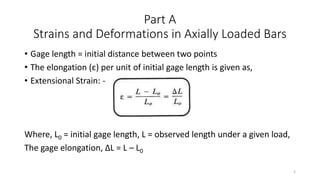
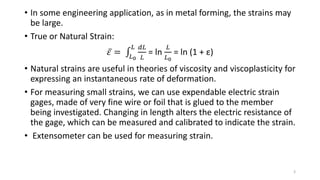
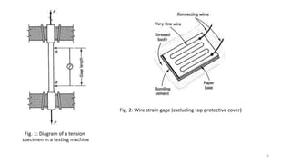
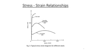
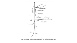
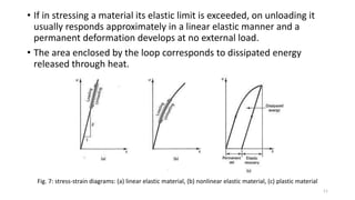
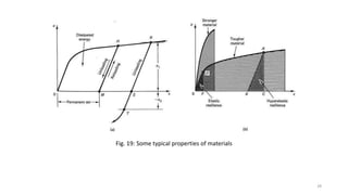
2. Part A
Strains and Deformations in Axially Loaded Bars
• Gage length = initial distance between two points
• The elongation (ε) per unit of initial gage length is given as,
• Extensional Strain: -
Where, L0 = initial gage length, L = observed length under a given load,
The gage elongation, ΔL = L – L0
2

3. • In some engineering application, as in metal forming, the strains may
be large.
• True or Natural Strain:
𝜀 = 𝐿0
𝐿 𝑑𝐿
𝐿
= ln
𝐿
𝐿0
= ln (1 + ε)
• Natural strains are useful in theories of viscosity and viscoplasticity for
expressing an instantaneous rate of deformation.
• For measuring small strains, we can use expendable electric strain
gages, made of very fine wire or foil that is glued to the member
being investigated. Changing in length alters the electric resistance of
the gage, which can be measured and calibrated to indicate the strain.
• Extensometer can be used for measuring strain.
3

4. Fig. 2: Wire strain gage (excluding top protective cover)
Fig. 1: Diagram of a tension
specimen in a testing machine
4

5. Stress - Strain Relationships
Fig. 3: Typical stress-strain diagrams for different steels
5

6. Fig. 4: Typical stress-strain diagrams for different materials
6

7. • Steel and Aluminum exhibit ductile behavior, and a fracture occurs
only after a considerable amount of deformation.
• These failures occur primarily due to slip in shear along the planes
forming approximately 45° angles with the axis of the load.
• A typical “cup and cone” fracture may be detected at fracture planes.
• In Fig. 5(b) , the upper curve represents some brittle tool steels or
concrete in tension, the middle one of aluminum alloys or plastics,
and the lower curve represents stress- strain characteristics of rubber.
• The terminal point of curve represents complete failure (rupture) of a
specimen.
• Ductile - Materials capable of withstanding large strains without a
significant increase in stress.
• Brittle - converse of Ductile.
7

8. Fig. 5: stress- strain diagrams: (a) mild steel, (b) typical materials
8

9. • Some transverse contraction or expansion of a material takes place. In
materials like mild steel or aluminum, near the breaking point
‘necking’ can be observed.
• True Stress = Dividing the applied force at a given point in the test, by
the corresponding actual area of a specimen at the same instant.
• Hooke’s law = Up to some point as A, the relationship between stress
and strain may be said to be linear for all materials.
𝜎 = 𝜀𝐸
Where, E = elastic modulus or young’s modulus.
• The stress corresponds to point A is known as ‘elastic limit’.
• Elastic modulus is a definitive property of material.
• For all steels E at room temperature is between 29 × 106 to 30 × 106
psi, or 200 to 207 GPa.
9

10. • Anisotropic = materials having different physical properties in
different directions, e.g., single crystals and wood.
• The highest point B represents, the ‘ultimate strength’ of a material.
• Stress associate with the long plateau ab, is called the yield strength
of a material.
• At an essentially constant stress, strains 15 to 20 times those that
take place up to the proportional limit occur during yielding.
Fig. 6: Offset method of determining the
Yield strength of a material
10

11. • If in stressing a material its elastic limit is exceeded, on unloading it
usually responds approximately in a linear elastic manner and a
permanent deformation develops at no external load.
• The area enclosed by the loop corresponds to dissipated energy
released through heat.
Fig. 7: stress-strain diagrams: (a) linear elastic material, (b) nonlinear elastic material, (c) plastic material
11

12. • For ductile materials, stress-strain diagram obtained for short
compressions blocks are close to those found in tension.
• Brittle materials, such as cast iron and concrete are very weak in
tension but not in compression.
• Constitutive relations or laws = additional stress-strain relations to
assumption of linearly elastic behavior of material.
• Ideally plastic behavior = a large amount of unbounded deformation
can take place at a constant stress.
• Assumptions: the mechanical properties of the material are the same
in both tension and compression. During unloading, the material
behaves elastically.
• A stress can range and terminate anywhere between + 𝜎 𝑦𝑝 and
− 𝜎 𝑦𝑝.
12

13. Fig. 8: Idealized stress-strain diagrams: (a) rigid perfectly plastic material, (b) elastic - perfectly plastic material,
(c) Elastic – linearly hardening material
• Strain hardening = Beyond the elastic range, on an increase in strain,
many material resists additional stress.
13

14. • Ramberg and Osgood equation:
𝜀
𝜀0
=
𝜎
𝜎0
+
3
7
𝜎
𝜎0
𝑛
• The constants 𝜀0 and 𝜎0 correspond to the yield point, which for all
cases other than that of ideal plasticity, is found by the offset method.
• The exponent ‘n’ determines the shape of the curve.
Fig. 9: Ramberg - Osgood
stress - strain diagrams
14

15. • The Ramberg-Osgood equation is a continuous mathematical
function. An instantaneous or tangent modulus, Et =
𝑑𝜎
𝑑𝜀
can be
uniquely determined.
• A series of characteristic loops, referred as ‘hysteretic loops’
representing the dissipation of energy can be seen in Fig. 10
• Stress- strain diagram is strongly dependent on ambient temperature.
(Fig. 11)
• Creep = with time dependent behavior and a member subjected to a
constant stress, the elongations or deflections continue to increase
with time. (Fig. 12)
• Relaxation = The pre-stress in bolts of mechanical assemblies
operating at high temperature, as well as pre-stress in steel tendons
in reinforced concrete, tend to decrease gradually with time. (Fig. 13)
15

16. Fig. 10: Menegotto–Pinto computer model simulation Fig. 11: Effect of strain rate and temperature on
of cyclic stress-strain diagrams for steel stress-strain curves for 6061-T6 aluminum alloy
16

17. Fig. 12: creep in bar under constant stress Fig. 13: stress-relaxation curve
17

18. Deformation of Axially Loaded Bars
• The deflection characteristics of bars also provide necessary
information for determining the stiffness of systems in mechanical
vibration analysis.
• The normal strain, 𝜀 𝑥 in the x-direction is
𝑑𝑢
𝑑𝑥
, du is the axial
deformation of the infinitesimal element.
• Change in length between 2 points,
∆ = 0
𝐿
𝜀 𝑥 𝑑𝑥 =
𝑃 𝑥
𝐴 𝑥 𝐸 𝑥
𝑑𝑥 (∵ Hooke’s law)
18

19. Poisson’s ratio
• Lateral (transverse) expansion or contraction to the direction of
applied force.
• For elastic, isotropic and homogeneous materials,
𝜈 =
𝑙𝑎𝑡𝑒𝑟𝑎𝑙 𝑠𝑡𝑟𝑎𝑖𝑛
𝑎𝑥𝑖𝑎𝑙 𝑠𝑡𝑟𝑎𝑖𝑛
= −
𝑙𝑎𝑡𝑒𝑟𝑎𝑙 𝑠𝑡𝑟𝑎𝑖𝑛
𝑎𝑥𝑖𝑎𝑙 𝑠𝑡𝑟𝑎𝑖𝑛
• Here axial strains are caused by uniaxial stress only.
• For some concretes 𝜈 = 0.1, for rubber 𝜈 = 0.5(maximum)
• The Poisson effect exhibited by materials causes no additional
stresses other than compressive or tensile unless the transverse
deformation is inhibited or prevented.
19

20. Thermal Strain and Deformation
• Thermal strain, 𝜀 𝑇 = 𝛼(𝑇 − 𝑇0)
• Where, 𝛼 = coefficient of thermal expansion
• The extensional deformation, ∆ 𝑇= 𝛼(𝑇 − 𝑇0)L
Saint-Venant’s Principle and Stress Concentrations
• In reality, applied forces often approximate concentrated forces, and
the cross section of members can change abruptly. This causes stress
and strain disturbances in the proximity of such forces and changes in
cross-section.
20

21. • The manner of force application on stresses is important only in the
vicinity of the region where the force is applied.
Fig. 14: Stress distribution near a concentrated force in a rectangular elastic plane
21

22. • Using Finite element method, The initial undeformed mesh into
which the planar block is arbitrarily subdivided, and the greatly
exaggerated deformed mesh caused by the applied force are shown
in Fig. 15.
Fig. 15: (a) undeformed and deformed mesh on an elastic plane, (b) 𝜎 𝑦 contours,
(c) Normal stress distributions at b/4 and b/2 below top.
22

23. • At bolt holes or changes in cross section, the maximum normal
stresses are finite, which depends only on the geometric proportions
of a member.
• Stress concentration factor (K) = The ratio of the maximum to the
average stress.
𝜎 𝑚𝑎𝑥 = 𝐾𝜎 𝑎𝑣 = 𝐾
𝑃
𝐴
Fig. 16: Stress concentration factor
23

24. Fig. 17: Stress concentration factors for flat bars in tension
24

25. Elastic Strain Energy for Uniaxial Strain
• Forces and deformations gives ‘internal work’ done in a body by
externally applied forces. It is stored in an elastic body as the ‘internal
elastic energy of dissipation’, or the ‘elastic strain energy’.
Fig. 18: (a) An element in uniaxial tension,
(b) a Hookean stress-strain diagram
25

26. • Strain energy density = strain energy stored in an elastic body per unit
volume of the material, ‘modulus of resilience’
𝑈0 =
𝑑𝑈
𝑑𝑉
=
𝜎 𝑥 𝜀 𝑥
2
=
𝜎 𝑥
2
2𝐸
𝑈 =
𝜎𝑥
2
2𝐸
𝑑𝑉
• Complementary energy = The corresponding area enclosed by the
inclined line and the vertical axis
26

27. • Toughness = material’s ability to absorb energy up to fracture.
• In the inelastic range, only a small part of the energy absorbed by a
material is recoverable. Most of the energy is dissipated in
permanently deforming the material and is lost in heat.
• The energy that may be recovered when a specimen has been
stressed to some point A as in Fig. 19 is represented by the triangle
ABC. Line AB of this triangle is parallel to line OD.
27

28. Fig. 19: Some typical properties of materials
28

29. Deflections by the Energy Method
• We are determining the deflection caused by the application of a
single axial force.
𝑈 = 𝑊𝑒 =
1
2
𝑃∆ =
𝑃2
𝐿
2𝐴𝐸
Dynamic and Impact Loads
• A freely falling weight, or a moving body, that strikes a structure
delivers ‘dynamic’ or ‘impact’ load or force.
29

30. • Idealizing Assumptions:
1. Materials behave elastically, and no dissipation of energy takes
place at the point of impact or at the supports owing to local
inelastic deformation of materials.
2. The inertia of the system resisting an impact may be neglected.
3. The deflection of the system is directly proportional to the
magnitude of the applied force whether a force is dynamically or
statistically applied.
• Consider a weight ‘W’, falling from the height ‘h’ striking a spring
having constant ‘k’.
30

31. Fig. 20: Behavior of an elastic system under an impact force
• Static deflection due to weight w, ∆ 𝑠𝑡=
𝑊
𝑘
• The maximum dynamic deflection, ∆ 𝑚𝑎𝑥=
𝑃 𝑑𝑦𝑛
𝑘
31

32. • Therefore, 𝑃𝑑𝑦𝑛 =
∆ 𝑚𝑎𝑥
∆ 𝑠𝑡
W
• External work can be equated to internal strain energy,
𝑊 ℎ + ∆ 𝑚𝑎𝑥 = 1
2
𝑃𝑑𝑦𝑛∆ 𝑚𝑎𝑥
• Simplifying, ∆ 𝑚𝑎𝑥 = ∆ 𝑠𝑡 1 + 1 +
2ℎ
∆ 𝑠𝑡
and 𝑃𝑑𝑦𝑛 = 𝑊 1 + 1 +
2ℎ
∆ 𝑠𝑡
• If, h is large compared to ∆ 𝑠𝑡, the impact factor is approximately equal
to
2ℎ
∆ 𝑠𝑡
32

33. Part B – Statically Indeterminate System
• Basic Concepts:
1. ‘Equilibrium conditions’ for the system must be assured both in
global and local sense.
2. ‘Geometric compatibility’ among the deformed parts of a body and
at the boundaries must be satisfied.
3. ‘Constitutive (stress-strain) relations’ for the materials of the system
must be complied with.
33

34. Force Method of Analysis
• On applying force P at B, reactions R1 and R2 develop at the ends and
the system deforms.
Fig. 21: Force (flexibility) method of elastic analysis for a statically indeterminate
Axially loaded bar
34

35. • If the flexibility of the lower elastic bar is f2, the deflection
∆0 = 𝑓2 𝑃
∆1 = 𝑓1 + 𝑓2 𝑅1
• The compatibility of deformations at A is then achieved by,
∆0 + ∆1 = 0
𝑅1 = −
𝑓2
𝑓1 + 𝑓2
𝑃
35

36. Introduction to Displacement Method
• The Stiffness, 𝑘𝑖 = 𝐴𝑖 𝐸𝑖 𝐿𝑖
−𝑘1∆ − 𝑘2∆ + 𝑃 = 0
∆ =
𝑃
𝑘1+𝑘2
• The equilibrium conditions for the
free-bodies at i nodes A and C are
𝑅1 = −
𝑘1
𝑘1+ 𝑘2
𝑃
𝑅2 = −
𝑘2
𝑘1+ 𝑘2
𝑃
Fig. 22: Displacement method of analysis for a
Statically indeterminate axially loaded bar
36

37. Displacement Method with Several DoF
• Consider a bar system consisting of three segments of variable
stiffness defined by their respective spring constants ki’s.
• Each node marked in the figure from 1 to 4, is permitted to displace
vertically in either direction. Therefore, 4 DoF (one DoF per node)
• With no deflection at the ends, we have statically indeterminate
problem.
• With the adopted sign convention, the bar segment extension
between the ith and the (i+1)th node is ∆𝑖 − ∆𝑖+1 .
• The internal tensile force = ∆𝑖 − ∆𝑖+1 𝑘𝑖
37

38. Fig. 23: Axially loaded bar with 4 DoF
38

39. • Equilibrium condition 𝐹𝑥 = 0 for each node.
• Node 1:
• Recasting these equations into the following form,
• We know either the deflections ∆𝑖’s or reactions Pi’s.
39

40. • Writing these equations in the matrix form,
• This is symmetric stiffness matrix. We can use computer programs for
solving these equations simultaneously.
40

41. Statically Indeterminate Non-linear problems
• Global equilibrium equation:
R1 + R2 + P = 0
• Compatibility at the juncture of two bar
segments. Ends A and C are held, Fig. 24: A bar of
nonlinear material
∆ 𝐴𝐵= −∆ 𝐵𝐶
• Using constitutive law, If the bar behavior is
linearly elastic,
𝑅1 𝐿1
𝐴1 𝐸1
= −
𝑅2 𝐿2
𝐴2 𝐸2
41

42. Alternative Differential Equation Approach for
Deflections
• The axial deflection u of a bar is determined by solving a first-order
differential, 𝜀 𝑥 =
𝑑𝑢
𝑑𝑥
=
𝜎
𝐸
=
𝑃
𝐴𝐸
𝑃 = 𝐴𝐸
𝑑𝑢
𝑑𝑥
• Consider a system as shown in Fig. 25
Fig. 25: Infinitesimal element of an axially loaded bar
42

43. 𝐹𝑥 = 0,
𝑑𝑃 + 𝑝 𝑥 𝑑𝑥 = 0
𝑑𝑃
𝑑𝑥
= −𝑝 𝑥
• The rate of change with x of the internal axial force P is equal to
negative of the applied force px.
• Now, assuming AE as constant,
𝑑
𝑑𝑥
𝑑𝑢
𝑑𝑥
=
1
𝐴𝐸
𝑑𝑃
𝑑𝑥
𝐴𝐸
𝑑2 𝑢
𝑑𝑥2
= −𝑝 𝑥
43