This chapter discusses approximate inference methods for probabilistic models where exact inference is intractable. It introduces variational inference as a deterministic approximation approach. Variational inference works by restricting the distribution of latent variables to a simpler family that makes computation and optimization easier. The chapter provides examples of using variational inference for Gaussian mixtures and univariate Gaussian models. It explains how to derive a variational lower bound and optimize it using an iterative procedure similar to EM.
This document discusses Granger causality and how to test for it. It provides the following key points:
1) Granger causality measures whether variable A occurs before variable B and helps predict B, but does not guarantee true causality. If A does not Granger cause B, one can be more confident A does not cause B.
2) To test for Granger causality, autoregressive models are developed with and without the variable being tested, and an F-test or t-test is used to see if adding the variable significantly lowers the residuals.
3) The document applies this to test if changes in loans Granger cause changes in deposits using quarterly U.S. financial
This document summarizes key concepts from Chapter 8 of the book "Pattern Recognition and Machine Learning" regarding probabilistic graphical models. It introduces directed and undirected graphical models as visualization tools for probabilistic relationships between random variables. It provides examples of Bayesian networks and conditional independence. Key points covered include using graphs to factorize joint probabilities, the d-separation criteria for identifying conditional independence based on a graph, and applying these concepts to linear Gaussian models and discrete variable models.
Logistic Regression: Predicting The Chances Of Coronary Heart DiseaseMichael Lieberman
Logistic regression is used to predict the probability of an event occurring based on multiple predictor variables. This document discusses using logistic regression to predict the risk of coronary heart disease based on factors like smoking, cholesterol levels, body mass index, gender, age, and physical activity. It finds that smoking and high cholesterol levels are the highest risk factors for heart disease. The odds ratio is used to interpret the results, showing smokers have a 2.4 times higher risk than non-smokers. Examples estimate an inactive smoker's risk at 18% over 10 years, versus practically no risk for a healthy older man.
Time series decomposition involves breaking down a time series into various components: trend, seasonality, and error/noise. There are different decomposition models such as additive and multiplicative. Smoothing methods like moving averages are used to estimate the trend-cycle component by reducing random variation. Box-Jenkins models combine autoregressive (AR) and moving average (MA) terms to model time series, and involve identification, estimation, and diagnostic stages.
This document discusses recent developments in causal inference methods. It contains summaries of talks on several causal inference topics:
1. Miguel Hernan discusses the g-formula approach and inverse probability weighting for estimating causal effects under confounding.
2. Judith Lok discusses marginal structural models and g-estimation of structural nested models for longitudinal data, which allow controlling for time-varying confounding.
3. James Robins discusses single world intervention graphs for representing counterfactuals and the g-formula for estimating effects of dynamic treatment regimes.
4. Tyler VanderWeele discusses approaches for causal mediation analysis, including the difference method and natural direct and indirect effects.
The document discusses different types of moving averages used for demand forecasting, including simple moving average, weighted moving average, and exponential weighted moving average. An exponential weighted moving average assigns greater weight and importance to more recent data points compared to older data. The exponential weighted moving average model was adapted by Holt and Winter to include a trend term that allows it to capture changes over time. The model calculates the weighted average using a smoothing factor lambda between 0 and 1, with larger lambda values giving more weight to recent data.
Holt-Winters forecasting allows users to smooth a time series and use data to forecast selected areas. Exponential smoothing assigns decreasing weights and values against historical data to decrease the value of the weight for the older data, so more recent historical data is assigned more weight in forecasting than older results. The right augmented analytics provides user-friendly application of this method and allow business users to leverage this powerful tool.
The document provides an overview of multiple linear regression (MLR). MLR allows predicting a dependent variable from multiple independent variables. It extends simple linear regression by incorporating additional predictors. Key points covered include: purposes of MLR for explanation and prediction; assumptions of the method; interpreting R-squared values; comparing unstandardized and standardized regression coefficients; and testing the statistical significance of predictors.
Interpreting deep learning and machine learning models is not just another regulatory burden to be overcome. Scientists, physicians, researchers, and analyst that use these technologies for their important work have the right to trust and understand their models and the answers they generate. This talk is an overview of several techniques for interpreting deep learning and machine learning models and telling stories from their results.
Speaker: Patrick Hall is a Data Scientist and Product Engineer at H2O.ai. He’s also an Adjunct Professor at George Washington University for the Department of Decision Sciences. Prior to joining H2O, Patrick spent many years as a Senior Data Scientist SAS and has worked with many Fortune 500 companies on their data science and machine learning problems. https://www.linkedin.com/in/jpatrickhall
The document discusses concepts in social network analysis including measuring networks through embedding measures and positions/roles of nodes. It covers network measures such as reciprocity, transitivity, clustering, density, and the E-I index. It also discusses positions like structural equivalence and regular equivalence and how to compute positional similarity through adjacency matrices.
This document provides an introduction to logistic regression. It outlines key features such as using a logistic function to model a binary dependent variable that can take on values of 0 or 1. Logistic regression is a linear method that uses the logistic function to transform predictions. The document discusses applications in machine learning, medical science, social science, and industry. It also provides details on logistic regression models, including converting linear variables to logistic variables using a sigmoid function and examining the effects of varying the logistic growth and midpoint parameters on the logistic regression curve.
Businesses use forecasting extensively to make predictions such as demand, capacity, budgets and revenue. Among these different forecasting models identifying seasonal patterns in data can go a long way by providing seasonal insights to the business decision makers so that they can strategist for seasonal effects.
Applying Statistical Modeling and Machine Learning to Perform Time-Series For...PyData
Forecasting time-series data has applications in many fields, including finance, health, etc. There are potential pitfalls when applying classic statistical and machine learning methods to time-series problems. This talk will give folks the basic toolbox to analyze time-series data and perform forecasting using statistical and machine learning models, as well as interpret and convey the outputs.
Variational Autoencoder를 여러 가지 각도에서 이해하기 (Understanding Variational Autoencod...Haezoom Inc.
인공신경망을 이용한 generative model로서 많은 관심을 받고 있는 Variational Autoencoder (VAE)를 보다 잘 이해하기 위해서, 여러 가지 재미있는 관점에서 바라봅니다. VAE 및 머신러닝 일반에 지식을 가지고 있는 청중을 대상으로 진행된 세미나 자료입니다. 현장에서 구두로 설명된 부분은 슬라이드의 회색 박스에 보충설명을 적어두었습니다.
Similar to Chapter 16 structured probabilistic models for deep learning - 2 (7)
Photo wake up - 3d character animation from a single photoKyeongUkJang
The document describes the steps involved in animating a 3D character model from a single photo. It involves detecting the person in the photo using Faster R-CNN, estimating their 2D pose, segmenting the person from the background, fitting the SMPL body model to generate a rigged 3D mesh, correcting head pose and texturing the mesh to create a 3D animated character. The method aims to overcome limitations of prior work and produce more accurate 3D character animations from just a single image.
This document summarizes the t-SNE technique for visualizing high-dimensional data in two or three dimensions. It explains that t-SNE is an advanced version of Stochastic Neighbor Embedding (SNE) that can better preserve local and global data structures compared to linear dimensionality reduction methods. The document outlines how t-SNE converts Euclidean distances between data points in high-dimensions to conditional probabilities representing similarity. It also discusses the "crowding problem" that occurs when mapping high-dimensional data to low-dimensions, and how t-SNE addresses this issue.
Chapter 16 structured probabilistic models for deep learning - 2
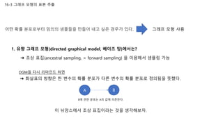
1. 1. 유향 그래프 모형(directed graphical model, 베이즈 망)에서는?
이 뉘앙스에서 조상 표집이라는 것을 생각해보자.
DGM을 다시 리마인드 하면
16-3 그래프 모형의 표본 추출
그래프 모형 사용
➔ 조상 표집(ancestral sampling, = forward sampling) 을 이용해서 샘플링 가능
➔ 화살표의 방향은 한 변수의 확률 분포가 다른 변수의 확률 분포로 정의됨을 뜻했다.
A B
B에 관한 분포는 A의 값에 의존한다.
어떤 확률 분포로부터 임의의 샘플들을 만들어 내고 싶은 경우가 있다.
1. 유향 그래프 모형(directed graphical model, 베이즈 망)에서는?
이 뉘앙스에서 조상 표집이라는 것을 생각해보자.
DGM을 다시 리마인드 하면
16-3 그래프 모형의 표본 추출
그래프 모형 사용
➔ 조상 표집(ancestral sampling, = forward sampling) 을 이용해서 샘플링 가능
➔ 화살표의 방향은 한 변수의 확률 분포가 다른 변수의 확률 분포로 정의됨을 뜻했다.
A B
B에 관한 분포는 A의 값에 의존한다.
어떤 확률 분포로부터 임의의 샘플들을 만들어 내고 싶은 경우가 있다.
2. 16-3 그래프 모형의 표본 추출
1) 3 개의 변수로 이루어진 결합 확률 분포 p(!" … !$), A~C까지 있다고 가정해보자
A B
C
2) 그래프가 주어졌을 때 각각의 노드에 번호를 붙인다.
- 이 때 자식 노드는 부모 노드보다 더 큰 번호를 부여한다.(위상 정렬)
A B
C1 2
3
조상 표집(ancestral sampling)
A B
C1 2
?
D
?
- 이렇게 순서가 여러 가지 나올 수도 있는데
그런 경우 유효 위상 순서 중 어떤 것도 가능하다.
3. A B
C1 2
3
16-3 그래프 모형의 표본 추출
조상 표집(ancestral sampling)
3) 그 순서에 따라 노드를 방문해 표본을 추출한다. 부모 ⇒ 자식
➔ 가장 먼저 p $% 분포로부터 &$% 을 추출
➔ 다음 노드 접근 p $'|$% 분포에서 샘플 추출
➔ 차례대로 노드를 방문하여 마지막 &$) 의 샘플을 생성
➔ 최종적으로 샘플(&$% … &$))을 얻게 된다.
핵심 : 이전 노드와의 조건부 분포로부터 표본을 추출한다.
4. 16-3 그래프 모형의 표본 추출
조상 표집(ancestral sampling)
3) 그 순서에 따라 노드를 방문해 표본을 추출한다. 부모 ⇒ 자식
➔ 가장 먼저 p $% 분포로부터 &$% 을 추출
➔ 다음 노드 접근 p $'|$% 분포에서 샘플 추출
➔ 차례대로 노드를 방문하여 마지막 &$) 의 샘플을 생성
➔ 최종적으로 샘플(&$% … &$))을 얻게 된다.
Alarm
JohnCalls MaryCalls
Buglary Earthquake
P(B)=0.001 P(E)=0.002
B E P(A|B,E)
T T 0.95
T F 0.94
F T 0.29
F F 0.001
A P(J|A)
T 0.90
F 0.05
A P(M|A)
T 0.70
F 0.01
5. A B
C1 2
3
16-3 그래프 모형의 표본 추출
조상 표집(ancestral sampling)
3) 그 순서에 따라 노드를 방문해 표본을 추출한다. 부모 ⇒ 자식
➔ 가장 먼저 p $% 분포로부터 &$% 을 추출
➔ 다음 노드 접근 p $'|$% 분포에서 샘플 추출
➔ 차례대로 노드를 방문하여 마지막 &$) 의 샘플을 생성
➔ 최종적으로 샘플(&$% … &$))을 얻게 된다.
핵심 : 이전 노드와의 조건부 분포로부터 표본을 추출한다.
단점
- 유향 그래프 모형에서만 적용할 수 있다.
- 찾아보니 요즘은 잘 안쓰는 방식이라고 한다.
6. 2. 무향 그래프 모형(undirected graphical model, 마르코프 망)에서의 표본 추출은?
16-3 그래프 모형의 표본 추출
➔ 모든 변수가 다른 모든 변수와 상호작용하므로
➔ 표집 과정의 시작 지점이 명확하지 않음
➔ 조상 표집(ancestral sampling)은 사용 불가
➔ 가장 간단한 접근 방식 깁스 샘플링(Gibbs sampling)
깁스 샘플링(Gibbs sampling)
➔ 마코프 연쇄 몬테카를로 방법의 일종(17장에서 자세히 다룰 예정)
➔ 간략하게만 어떤 것인지 다루고 넘어간다.
1) 3개의 확률변수의 결합확률분포 p(!", !$, !%) 로부터 1개의 표본을 얻으려고 할 때 깁스 샘플링 절차
7. 16-3 그래프 모형의 표본 추출
(1) 임의의 표본 !"=(#$
"
, #&
"
, #'
"
)을 선택한다.
(2) 현재 주어진 표본 !"
의 #&
"
, #'
"
를 고정한다.
(3) 첫번째 기존 #$
"
를 대체할 새로운 값 #$
$
을 p(#$
$
|#&
"
, #'
"
) 확률로 뽑는다.
(4) #$
$
, #'
"
을 고정 한다.
(5) #&
"
을 대체할 새로운 값 #&
$
을 p(#&
$
|#$
$
, #'
"
)
(6) 같은 방법으로 이번에는 #$
$
, #&
$
를 고정한다.
(7) 최종적으로 구한 !$
= (#$
$
, #&
$
, #'
$
)이다.
1) 3개의 확률변수의 결합확률분포 p(#$, #&, #') 로부터 1개의 표본을 얻으려고 할 때 깁스 샘플링 절차
깁스 샘플링(Gibbs sampling)
#$
,
, #&
,
, #'
,
#$
,-$
, #&
,
, #'
,
#$
,-$
, #&
,-$
, #'
,
#$
,-$
, #&
,-$
, #'
,-$
핵심 : 변수 #.에 대해 샘플링 ⇒ 그 이외의 모든 변수를 조건으로 한 조건부 분포로부터 그 변수의 값을 샘플링한다.
11. 16-3 그래프 모형의 표본 추출
깁스 샘플링(Gibbs sampling)
- 점근적으로 이런 과정을 반복하면 desired distribution에 수렴한다.
- high dimensional distribution에서 sampling하는데 매우 유용하다.
- 17장에서 좀 더 자세하게 다루도록 한다.
12. 샘플링을 통해 데이터를 생성하는 것
확률 모형을 만든다는 것
데이터 확률 모형을 학습해야 하는 것
input data의 분포를 정확하게 포착하면 할 수록 좋은 것
16-5 종속 관계의 학습
13. 샘플링을 통해 데이터를 생성하는 것
확률 모형을 만든다는 것
데이터 확률 모형을 학습해야 하는 것
input data의 분포를 정확하게 포착하면 할 수록 좋은 것
그런데 input data는 서로 다른 feature 사이에 관계(ex 종속 관계)가 존재할 때가 많다.
16-5 종속 관계의 학습
14. 샘플링을 통해 데이터를 생성하는 것
확률 모형을 만든다는 것
데이터 확률 모형을 학습해야 하는 것
input data의 분포를 정확하게 포착하면 할 수록 좋은 것
그런데 input data는 서로 다른 feature 사이에 관계(ex 종속 관계)가 존재할 때가 많다.
따라서 의존성을 잘 포착해서 그래프 모형을 만들어야 좋은 그래프 모형
16-5 종속 관계의 학습
15. 16-5 종속 관계의 학습
!"
!#
ℎ
“hidden” variable 1) !"와 !# 사이의 간접 종속 관계가 있는지 궁금하다.
2) !"와 ℎ 사이의 직접 종속 관계 확인
3) !#와 ℎ 사이의 직접 종속 관계를 통해서 확인한다.
그런 관계를 포착하는 방법 예시
“visible” variable(= input data)
16. 16-5 종속관계의 학습(Learning about Dependencies)
➔ 다양한 방법이 있지만 general 한 방법을 이야기하자
data set three example network structures
그래프 모형을 만드는 방법
17. 16-5 종속관계의 학습(Learning about Dependencies)
➔ to define a scoring function that tells us, for each of these network structures,
how good it is relative to the data
1) Likelihood Scores
2) Bayesian Scores
➔ we have the goal of searching for a network structure that maximizes the score.
data set three example network structures
18. 16-5 종속관계의 학습(Learning about Dependencies)
나올법한 질문
1) 변수가 엄청 많으면 만들 수 있는 structure의 경우의 수도 많을텐데 모든 case에 대
해서 전부 다해봐? 어떻게 초기 structure를 설정?
data set three example network structures
19. 16-5 종속관계의 학습(Learning about Dependencies)
나올법한 질문
1) 변수가 엄청 많으면 만들 수 있는 structure의 경우의 수도 많을텐데 모든 case에 대
해서 전부 다해봐? 어떻게 초기 structure를 설정?
➔ 교재 왈 : 모든 변수를 연결하는 것은 일반적으로 비현실적이므로 서로 밀접하게 연
관된 변수만 연결하고 그 외의 변수들 사이의 edge는 생략한 그래프를 만들도록 한다.
data set three example network structures
20. 16-4 구조적 모형화의 장점
1. 확률 분포의 표현 비용, 학습과 추론 비용이 극적으로 줄어든다.
➔ The primary advantage of using structured probabilistic models is that
they allow us to dramatically reduce the cost of representing probability distributions
as well as learning and inference.
➔ 앞서 인준형이 이야기했던 부분
2. 학습으로 얻은 지식의 표현과 기존 지식에 기초한 추론으로 얻은 지식의 표현을 명시적으로 분리할 수 있다.
➔ 조금 우회해서 해석해보면
21. 16-4 구조적 모형화의 장점
1. 확률 분포의 표현 비용, 학습과 추론 비용이 극적으로 줄어든다.
➔ The primary advantage of using structured probabilistic models is that
they allow us to dramatically reduce the cost of representing probability distributions
as well as learning and inference.
2. 학습으로 얻은 지식의 표현과 기존 지식에 기초한 추론으로 얻은 지식의 표현을 명시적으로 분리할 수 있다.
➔ variable들의 structure(서로 어떤 위계가 있는지)를 발견하는 것 자체가 의미가 있는 상황이 있을 수 있다.
➔ scientific or biological data sets
➔ 변수들 사이에 interrelationship을 발견하는 것이 domain을 더 잘 이해하는데 도움을 줄 수 있다.
➔ ex) 특정 환자가 가지고 있을 만한 질병을, 주어진 의료 진단 자료를 조건으로 하여 확률 모형으로
알아 낼 수 있다.
➔ 확률 모형의 주된 용도는 변수들 사이의 관계를 질의 하는 것
22. 16-7 구조적 확률 모형에 대한 심측 학습 접근 방식, 제한 볼츠만 기계(Restricted Boltzmann machine)
RBM은 그래프 모형에 대한 전형적인 심층 학습 접근 방식이라고 한다.
RBM이 뭔데? (20장에서 다루기에 정말 정말 간단하게)
오토인코더랑 같은 목적 =>
But 그 방식이 다르다.(앞에서 이야기한 에너지 모델)
23. 16-7 구조적 확률 모형에 대한 심측 학습 접근 방식, 제한 볼츠만 기계(Restricted Boltzmann machine)
RBM은 그래프 모형에 대한 전형적인 심층 학습 접근 방식이라고 한다.
어떠한 x가 있을 확률은 E(x), 즉 에너지 함수에 반비례한다.
에너지를 학습하는 것이 RBM의 목적
에너지 함수라는 건 w, b, a의 식으로 구성됨
24. 16-7 구조적 확률 모형에 대한 심측 학습 접근 방식, 제한 볼츠만 기계(Restricted Boltzmann machine)
RBM이 뭔데? (20장에서 다루기에 정말 정말 간단하게)
) ( 0 2 . ==
B R M
RBM은 그래프 모형에 대한 전형적인 심층 학습 접근 방식이라고 한다.