CostVolumeProfitAnalysis.pptx

1. *Cost Volume Profit Analysis
Plans fail for lack of counsel, but with many advisers they succeed.
Proverbs 15:22

2. Cost-volume-profit analysis (CVP analysis) is
a powerful tool for planning and decision
making. Because CVP analysis emphasizes
the interrelationships of costs, quantity sold,
and price, it brings together all of the
financial information of the firm. CVP
analysis can be a valuable tool in identifying
the extent and magnitude of the economic
trouble a company is facing and helping
pinpoint the necessary solution.

3. Cost-volume-profit (CVP) analysis is a
technique for analyzing how costs and
profits change with the volume of
production and sales. It is also called the
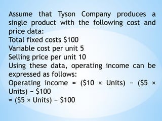
Break-even analysis. CVP analysis assumes
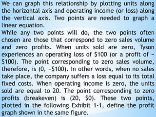
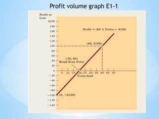
that selling prices and variable costs are
constant per unit at all volumes of sales and
that fixed costs remain fixed at all levels of
activity.

4. The starting point of presenting the
CVP analysis is to find the firm’s
break-even point in units sold. The
break-even point is the point of zero
profit. Two frequently used
approaches to finding the break-even
point in units are the operating
income approach and the contribution
margin approach.

5. CVP analysis focuses on the factors that
effect a change in the components of
profit. Because we are looking at CVP
analysis in terms of units sold, we need to
determine the fixed and variable
components of cost and revenue with
respect to units. It is important to realize
that we are focusing on the firm as a
whole. Therefore, the costs we are
talking about are all costs of the
company: manufacturing, marketing, and
administrative.

6. Thus, when we say variable costs,
we mean all costs that increase as
more units are sold, including direct
materials, direct labour, variable
overhead, and variable selling and
administrative costs. Similarly, fixed
costs include fixed overhead and
fixed selling and administrative
expenses.

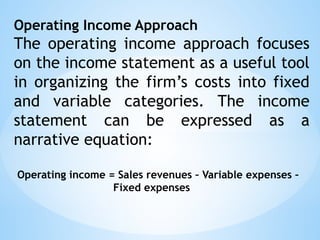
7. Operating Income Approach
The operating income approach focuses
on the income statement as a useful tool
in organizing the firm’s costs into fixed
and variable categories. The income
statement can be expressed as a
narrative equation:
Operating income = Sales revenues – Variable expenses –
Fixed expenses

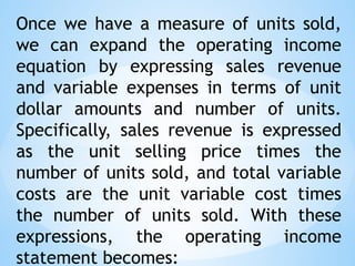
8. Once we have a measure of units sold,
we can expand the operating income
equation by expressing sales revenue
and variable expenses in terms of unit
dollar amounts and number of units.
Specifically, sales revenue is expressed
as the unit selling price times the
number of units sold, and total variable
costs are the unit variable cost times
the number of units sold. With these
expressions, the operating income
statement becomes:

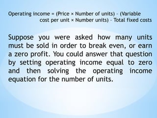
9. Operating income = (Price × Number of units) – (Variable
cost per unit × Number units) – Total fixed costs
Suppose you were asked how many units
must be sold in order to break even, or earn
a zero profit. You could answer that question
by setting operating income equal to zero
and then solving the operating income
equation for the number of units.

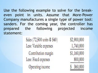
10. Use the following example to solve for the break-
even point in units. Assume that More-Power
Company manufactures a single type of power tool:
sanders. For the coming year, the controller has
prepared the following projected income
statement:

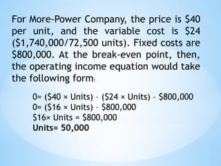
11. For More-Power Company, the price is $40
per unit, and the variable cost is $24
($1,740,000/72,500 units). Fixed costs are
$800,000. At the break-even point, then,
the operating income equation would take
the following form:
0= ($40 × Units) – ($24 × Units) – $800,000
0= ($16 × Units) – $800,000
$16× Units = $800,000
Units= 50,000

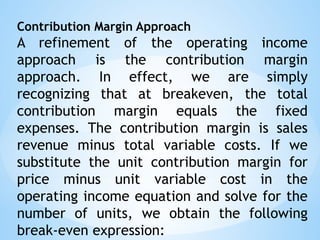
12. Contribution Margin Approach
A refinement of the operating income
approach is the contribution margin
approach. In effect, we are simply
recognizing that at breakeven, the total
contribution margin equals the fixed
expenses. The contribution margin is sales
revenue minus total variable costs. If we
substitute the unit contribution margin for
price minus unit variable cost in the
operating income equation and solve for the
number of units, we obtain the following
break-even expression:

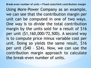
13. Break-even number of units = Fixed costs/Unit contribution margin
Using More-Power Company as an example,
we can see that the contribution margin per
unit can be computed in one of two ways.
One way is to divide the total contribution
margin by the units sold for a result of $16
per unit ($1,160,000/72,500). A second way
is to compute price minus variable cost per
unit. Doing so yields the same result, $16
per unit ($40 – $24). Now, we can use the
contribution margin approach to calculate
the break-even number of units.

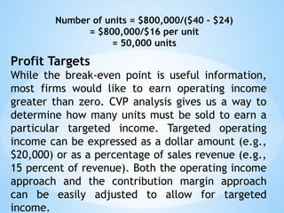
14. Number of units = $800,000/($40 – $24)
= $800,000/$16 per unit
= 50,000 units
Profit Targets
While the break-even point is useful information,
most firms would like to earn operating income
greater than zero. CVP analysis gives us a way to
determine how many units must be sold to earn a
particular targeted income. Targeted operating
income can be expressed as a dollar amount (e.g.,
$20,000) or as a percentage of sales revenue (e.g.,
15 percent of revenue). Both the operating income
approach and the contribution margin approach
can be easily adjusted to allow for targeted
income.

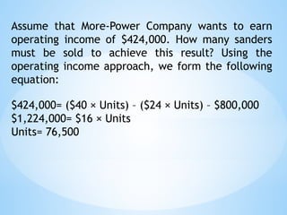
15. Assume that More-Power Company wants to earn
operating income of $424,000. How many sanders
must be sold to achieve this result? Using the
operating income approach, we form the following
equation:
$424,000= ($40 × Units) – ($24 × Units) – $800,000
$1,224,000= $16 × Units
Units= 76,500

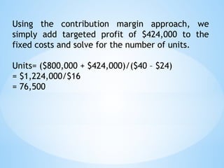
16. Using the contribution margin approach, we
simply add targeted profit of $424,000 to the
fixed costs and solve for the number of units.
Units= ($800,000 + $424,000)/($40 – $24)
= $1,224,000/$16
= 76,500

17. Graphical representation of CVP relationships
Visual portrayals may further our
understanding of CVP relationships. A
graphical representation can help managers
see the difference between variable cost and
revenue. It may also help managers
understand quickly what impact an increase
or decrease in sales will have on the break-
even point. Two basic graphs, the profit-
volume graph and the cost-volume-profit
graph, are presented.

18. The Profit-Volume Graph
A profit-volume graph visually portrays the
relationship between profits and sales
volume. The profit-volume graph is the
graph of the operating income equation:
[Operating income= (Price × Units) − (Unit
variable cost × Units) − Fixed costs].
In this graph, operating income (profit) is the
dependent variable, and units is the
independent variable. Usually, values of the
independent variable are measured along
the horizontal axis and values of the
dependent variable along the vertical axis.

19. Assume that Tyson Company produces a
single product with the following cost and
price data:
Total fixed costs $100
Variable cost per unit 5
Selling price per unit 10
Using these data, operating income can be
expressed as follows:
Operating income = ($10 × Units) − ($5 ×
Units) − $100
= ($5 × Units) − $100

20. We can graph this relationship by plotting units along
the horizontal axis and operating income (or loss) along
the vertical axis. Two points are needed to graph a
linear equation.
While any two points will do, the two points often
chosen are those that correspond to zero sales volume
and zero profits. When units sold are zero, Tyson
experiences an operating loss of $100 (or a profit of −
$100). The point corresponding to zero sales volume,
therefore, is (0, −$100). In other words, when no sales
take place, the company suffers a loss equal to its total
fixed costs. When operating income is zero, the units
sold are equal to 20. The point corresponding to zero
profits (breakeven) is (20, $0). These two points,
plotted in the following Exhibit 1-1, define the profit
graph shown in the same figure.

21. Profit volume graph E1-1

22. The graph in Exhibit 1-1 can be used to assess
Tyson’s profit (or loss) at any level
of sales activity. For example, the profit associated
with the sale of 40 units can be read from the graph
by (1) drawing a vertical line from the horizontal
axis to the profit line and (2) drawing a horizontal
line from the profit line to the vertical axis. As
illustrated in Exhibit 1-1, the profit associated with
sales of 40 units is $100.
The profit-volume graph, while easy to interpret,
fails to reveal how costs change as sales volume
changes. An alternative approach to graphing can
provide this detail.

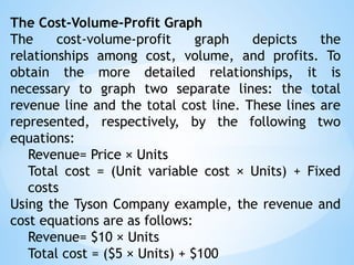
23. The Cost-Volume-Profit Graph
The cost-volume-profit graph depicts the
relationships among cost, volume, and profits. To
obtain the more detailed relationships, it is
necessary to graph two separate lines: the total
revenue line and the total cost line. These lines are
represented, respectively, by the following two
equations:
Revenue= Price × Units
Total cost = (Unit variable cost × Units) + Fixed
costs
Using the Tyson Company example, the revenue and
cost equations are as follows:
Revenue= $10 × Units
Total cost = ($5 × Units) + $100

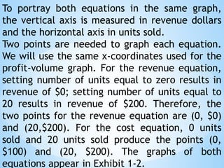
24. To portray both equations in the same graph,
the vertical axis is measured in revenue dollars
and the horizontal axis in units sold.
Two points are needed to graph each equation.
We will use the same x-coordinates used for the
profit-volume graph. For the revenue equation,
setting number of units equal to zero results in
revenue of $0; setting number of units equal to
20 results in revenue of $200. Therefore, the
two points for the revenue equation are (0, $0)
and (20,$200). For the cost equation, 0 units
sold and 20 units sold produce the points (0,
$100) and (20, $200). The graphs of both
equations appear in Exhibit 1-2.

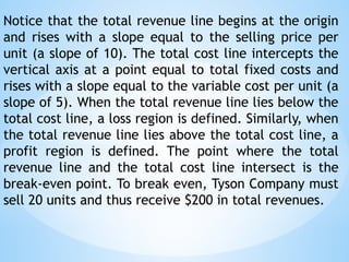
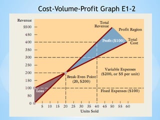
25. Notice that the total revenue line begins at the origin
and rises with a slope equal to the selling price per
unit (a slope of 10). The total cost line intercepts the
vertical axis at a point equal to total fixed costs and
rises with a slope equal to the variable cost per unit (a
slope of 5). When the total revenue line lies below the
total cost line, a loss region is defined. Similarly, when
the total revenue line lies above the total cost line, a
profit region is defined. The point where the total
revenue line and the total cost line intersect is the
break-even point. To break even, Tyson Company must
sell 20 units and thus receive $200 in total revenues.

26. Cost-Volume-Profit Graph E1-2

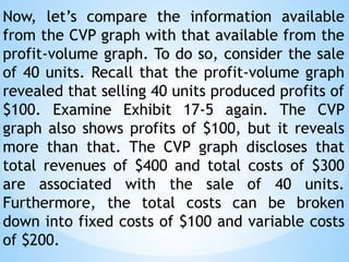
27. Now, let’s compare the information available
from the CVP graph with that available from the
profit-volume graph. To do so, consider the sale
of 40 units. Recall that the profit-volume graph
revealed that selling 40 units produced profits of
$100. Examine Exhibit 17-5 again. The CVP
graph also shows profits of $100, but it reveals
more than that. The CVP graph discloses that
total revenues of $400 and total costs of $300
are associated with the sale of 40 units.
Furthermore, the total costs can be broken
down into fixed costs of $100 and variable costs
of $200.

28. The CVP graph provides revenue and cost
information not provided by the profit-
volume graph. Unlike the profit-volume
graph, some computation is needed to
determine the profit associated with a
given sales volume.
Nonetheless, because of the greater
information content, managers are likely
to find the CVP graph a more useful tool.

29. Assumptions of Cost-Volume-Profit Analysis
The profit-volume and cost-volume-profit graphs rely
on some important assumptions:
1.The analysis assumes a linear revenue function and a
linear cost function.
2.The analysis assumes that price, total fixed costs,
and unit variable costs can be accurately identified
and remain constant over the relevant range (recall
that the relevant range is the range over which the
cost relationship is valid).
3.The analysis assumes that what is produced is sold.
4.For multiple-product analysis, the sales mix is
assumed to be known.
5.The selling prices and costs are assumed to be
known with certainty.

30. MARGIN OF SAFETY
Actual sales volume will not be the same as budgeted sales
volume. Actual sales will probably either fall short of budget
or exceed budget. A useful analysis of business risk is to look
at what might happen to profit if actual sales volume is less
than budgeted.
The difference between budgeted sales volume and the
break-even sales volume is known as the margin of safety.
It is simply a measurement of how far sales can fall short of
budget before the business makes a loss. In this respect, a
large margin of safety indicates a low risk of making a loss,
whereas a small margin of safety might indicate a fairly high
risk of a loss. It therefore indicates the vulnerability of a
business to a fall in demand.

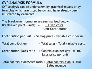
31. CVP ANALYSIS FORMULA
CVP analysis can be undertaken by graphical means or by
formulae which are listed below and have already been
illustrated by examples.
The break-even formulae are summarized below:
Break-even point (units) = Fixed costs
Unit Contribution
Contribution per unit = Selling price – variable cost per unit
Total contribution = Total sales – Total variable costs
Contribution/Sales ratio = Contribution per unit x 100
Sales price per unit
Total contribution/Sales ratio = Total contribution x 100
Sales revenue

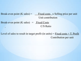
32. Break-even point (K sales) = Fixed costs x Selling price per unit
Unit contribution
Break-even point (K sales) = Fixed Costs
C/S Ratio
Level of sales to result in target profit (in units) = Fixed costs + T. Profit
Contribution per unit