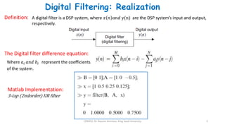
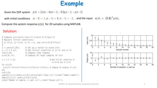
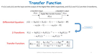
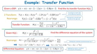
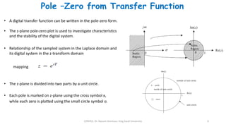
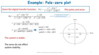
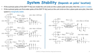
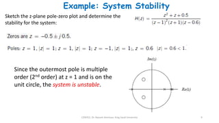
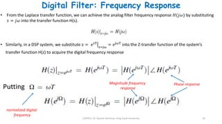
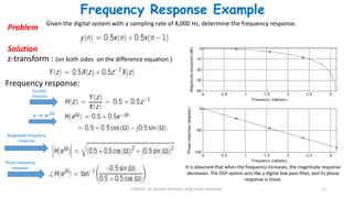
1) Digital filters are discrete-time systems that perform operations on sampled input signals. They are described by difference equations relating the current output to current and previous input/output values. 2) The transfer function of a digital filter relates the Z-transform of its input and output and can be used to analyze properties like poles, zeros, and stability. 3) The frequency response of a digital filter is obtained by substituting Z = e^jΩ into its transfer function and indicates how the filter affects different frequencies, determining its type (low-pass, high-pass, etc.).

1. Chapter 6
Digital Filters
CEN352, Dr. Nassim Ammour, King Saud University 1

2. CEN352, Dr. Nassim Ammour, King Saud University 2
Digital Filtering: Realization
The Digital filter difference equation:
Where 𝑎𝑖 𝑎𝑛𝑑 𝑏𝑖 represent the coefficients
of the system.
A digital filter is a DSP system, where 𝑥 𝑛 𝑎𝑛𝑑 y(n) are the DSP system’s input and output,
respectively.
Definition:
Matlab Implementation:
3-tap (2ndorder) IIR filter

3. CEN352, Dr. Nassim Ammour, King Saud University 3
Example
Given the DSP system
with initial conditions and the input
Compute the system response y(n) for 20 samples using MATLAB.
Solution:

4. CEN352, Dr. Nassim Ammour, King Saud University 4
Transfer Function
If 𝑥 𝑛 and 𝑦 𝑛 are the input and the output of the Digital filter (DSP) respectively, and 𝑋 𝑧 𝑎𝑛𝑑 𝑌 𝑧 are their Z-transforms,
Differential Equation:
Z-Transform:
Transfer Function:
Z-Transform

5. CEN352, Dr. Nassim Ammour, King Saud University 5
Example: Transfer Function
Given a DSP: Find the its transfer function H(z).
Z-Transform:
Z-transform on both sides
of the difference equation
Rearrange:
factoring Y(z) on the left side
and X(z) on the right side
Transfer Function:
Dividing the numerator and denominator by 𝑧2
Given H(z) : Find the difference equation of the system
Rearrange:
Applying the inverse z-transform
and using the shift property
Differential Equation:

6. CEN352, Dr. Nassim Ammour, King Saud University 6
Pole –Zero from Transfer Function
• A digital transfer function can be written in the pole-zero form.
• The z-plane pole-zero plot is used to investigate characteristics
and the stability of the digital system.
• Relationship of the sampled system in the Laplace domain and
its digital system in the z-transform domain
mapping:
• The z-plane is divided into two parts by a unit circle.
• Each pole is marked on z-plane using the cross symbol x,
while each zero is plotted using the small circle symbol o.

7. CEN352, Dr. Nassim Ammour, King Saud University 7
Example: Pole-zero plot
Plot poles and zeros
Given the digital transfer function:
multiplying the numerator
and denominator by 𝑧2
=
(𝑧 − 𝑧𝑒𝑟𝑜1)
(𝑧 − 𝑝𝑜𝑙𝑒1)(𝑧 − 𝑝𝑜𝑙𝑒2)
The system is stable.
The zeros do not affect
system stability.
𝑧𝑒𝑟𝑜1 = 0.5
𝑝𝑜𝑙𝑒1 = −0.6 + 𝑗0.3
𝑝𝑜𝑙𝑒2 = −0.6 − 𝑗0.3

8. CEN352, Dr. Nassim Ammour, King Saud University 8
System Stability (Depends on poles’ location)
• If the outmost poles of the DSP TF H(z) are inside the unit circle on the z-plane pole-zero plot, then the system is stable.
• If the outmost poles are first-order poles of the DSP TF H(z) and on the unit circle on the z-plane pole-zero plot, then the
system is marginally stable.

9. CEN352, Dr. Nassim Ammour, King Saud University 9
Example: System Stability
Sketch the z-plane pole-zero plot and determine the
stability for the system:
Since the outermost pole is multiple
order (2nd order) at z = 1 and is on the
unit circle, the system is unstable.

10. CEN352, Dr. Nassim Ammour, King Saud University 10
Digital Filter: Frequency Response
• From the Laplace transfer function, we can achieve the analog filter frequency response 𝐻(𝑗𝜔) by substituting
𝑠 = 𝑗𝜔 into the transfer function H(s).
Magnitude frequency
response
Phase response
Putting
• Similarly, in a DSP system, we substitute z = esT
s=jω
= ejωT into the Z-transfer function of the system’s
transfer function H(z) to acquire the digital frequency response
normalized digital
frequency

11. CEN352, Dr. Nassim Ammour, King Saud University 11
Frequency Response Example
Given the digital system with a sampling rate of 8,000 Hz, determine the frequency response.
Solution
Problem
z-transform : (on both sides on the difference equation )
transfer
function
Frequency response:
𝑧 = 𝑒𝑗Ω
Magnitude frequency
response
Phase frequency
response It is observed that when the frequency increases, the magnitude response
decreases. The DSP system acts like a digital low-pass filter, and its phase
response is linear.

12. CEN352, Dr. Nassim Ammour, King Saud University 12
Digital Filter: Frequency Response –contd.
BASIC TYPES OF FILTERING
Pass-band Ripple
(frequency fluctuation)
parameter
Stop-band Ripple
(frequency fluctuation)
parameter
Pass-band cut-off
frequency
Stop-band cut-off
frequency
Low-pass filter (LPF)
High-pass filter (HPF)
Matlab: Frequency Response:

13. CEN352, Dr. Nassim Ammour, King Saud University 13
Digital Filter: Frequency Response –contd.
BASIC TYPES OF FILTERING
Lower stop-band
cut-off frequency Lower Pass-band
cut-off frequency
Higher stop-band
Cut-off frequency
Higher pass-band
Cut-off frequency
Band-stop filter (BSF)
Band-pass filter (BPF)