This document outlines the key topics covered in Chapter 2 of the book "Linear Algebra" by Jin Ho Lee. The chapter introduces fundamental concepts in linear algebra including scalars, vectors, matrices, and tensors. It describes operations on these objects such as matrix multiplication and vector dot products. Important matrix properties and special types of matrices like identity, inverse, diagonal, and symmetric matrices are defined. Linear dependence, spans, and vector spaces are discussed. Various vector and matrix norms are also introduced.

1. Chapter 2
Linear
Algebra
JIN HO LEE
2.1
2.2
2.3
2.4
2.5
2.6
2.7
2.8
2.9
2.10
2.11
2.12
.
.
.
.
.
.
.
.
.
.
.
.
.
.
.
.
.
.
.
.
.
.
.
.
.
.
.
.
.
.
.
.
.
.
.
.
.
.
.
.
Chapter 2 Linear Algebra
JIN HO LEE
2018-5-20
JIN HO LEE Chapter 2 Linear Algebra

2. Chapter 2
Linear
Algebra
JIN HO LEE
2.1
2.2
2.3
2.4
2.5
2.6
2.7
2.8
2.9
2.10
2.11
2.12
.
.
.
.
.
.
.
.
.
.
.
.
.
.
.
.
.
.
.
.
.
.
.
.
.
.
.
.
.
.
.
.
.
.
.
.
.
.
.
.
Contents
• 2.1 Scalars, Vectors, Matrices and Tensors
• 2.2 Multiplying Matrices and Vectors
• 2.3 Identity and Inverse Matrices
• 2.4 Linear Dependence and Span
• 2.5 Norms
• 2.6 Special Kinds of Matrices and Vectors
• 2.7 Eigendecomposition
• 2.8 Singular Value Decomposition
• 2.9 The Moore-Penrose Pseudoinverse
• 2.10 The Trace Operator
• 2.11 The Determinant
• 2.12 Example: Principal Components Analysis
JIN HO LEE Chapter 2 Linear Algebra

3. Chapter 2
Linear
Algebra
JIN HO LEE
2.1
2.2
2.3
2.4
2.5
2.6
2.7
2.8
2.9
2.10
2.11
2.12
.
.
.
.
.
.
.
.
.
.
.
.
.
.
.
.
.
.
.
.
.
.
.
.
.
.
.
.
.
.
.
.
.
.
.
.
.
.
.
.
2.1 Scalars, Vectors, Matrices and Tensors
□ Definitions
• Scalar : A scalar is just a single number.
• Vectors : A vector is an array of numbers. x 가
n-dimensional vector 라면 x1, x2, · · · , xn ∈ R 이 존재해서
x =





x1
x2
...
xn





로 표현 가능하다. x1, x2, · · · , xn 을 x의 entry라고 한다.
JIN HO LEE Chapter 2 Linear Algebra

4. Chapter 2
Linear
Algebra
JIN HO LEE
2.1
2.2
2.3
2.4
2.5
2.6
2.7
2.8
2.9
2.10
2.11
2.12
.
.
.
.
.
.
.
.
.
.
.
.
.
.
.
.
.
.
.
.
.
.
.
.
.
.
.
.
.
.
.
.
.
.
.
.
.
.
.
.
2.1 Scalars, Vectors, Matrices and Tensors
S 를 index set 이라고 하자. 예를 들어, x 의 dimension 이 7
이고 S = {1, 3, 6} 일 때, xS = {x1, x3, x6}를 의미한다. 또한
x−2 은 index 중 2가 아닌 x의 모든 entry 들의 집합을 의미한다.
즉, x−2 = {x1, x3, x4, x5, x6, x7}. 마찬가지로 x−S 는 index 가 S
의 원소가 아닌 x의 entry 들의 집합이다. 즉,
x−S = {x2, x4, x5, x7} 을 의미한다.
• Matrices : A matrix is a 2-dimensional array of numbers. If a
real-valued matrix A has a height of m and a width of n, then
we say that A ∈ Rm×n.
JIN HO LEE Chapter 2 Linear Algebra

5. Chapter 2
Linear
Algebra
JIN HO LEE
2.1
2.2
2.3
2.4
2.5
2.6
2.7
2.8
2.9
2.10
2.11
2.12
.
.
.
.
.
.
.
.
.
.
.
.
.
.
.
.
.
.
.
.
.
.
.
.
.
.
.
.
.
.
.
.
.
.
.
.
.
.
.
.
2.1 Scalars, Vectors, Matrices and Tensors
Sometimes we write
A = (Ai,j)1≤j≤n
1≤i≤m
it means that
A =



A1,1 A1,2 · · · A1,n
...
...
...
...
Am,1 Am,2 · · · Am,n



matrix A의 i 번째 행을 Ai,: 로 표기한다. 마찬가지로 A의 j 번째
열을 A:,j 로 표기한다.
JIN HO LEE Chapter 2 Linear Algebra

6. Chapter 2
Linear
Algebra
JIN HO LEE
2.1
2.2
2.3
2.4
2.5
2.6
2.7
2.8
2.9
2.10
2.11
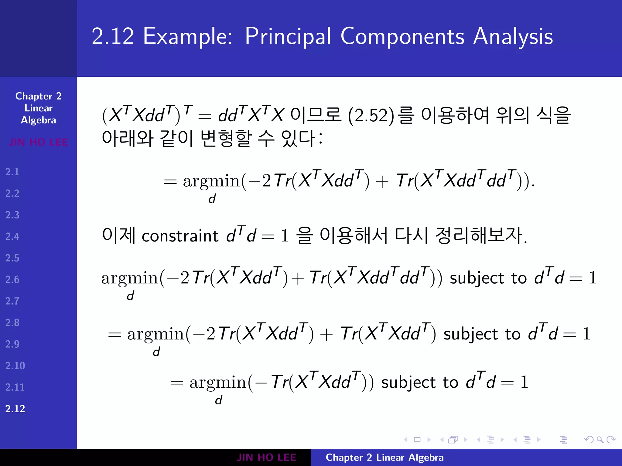
2.12
.
.
.
.
.
.
.
.
.
.
.
.
.
.
.
.
.
.
.
.
.
.
.
.
.
.
.
.
.
.
.
.
.
.
.
.
.
.
.
.
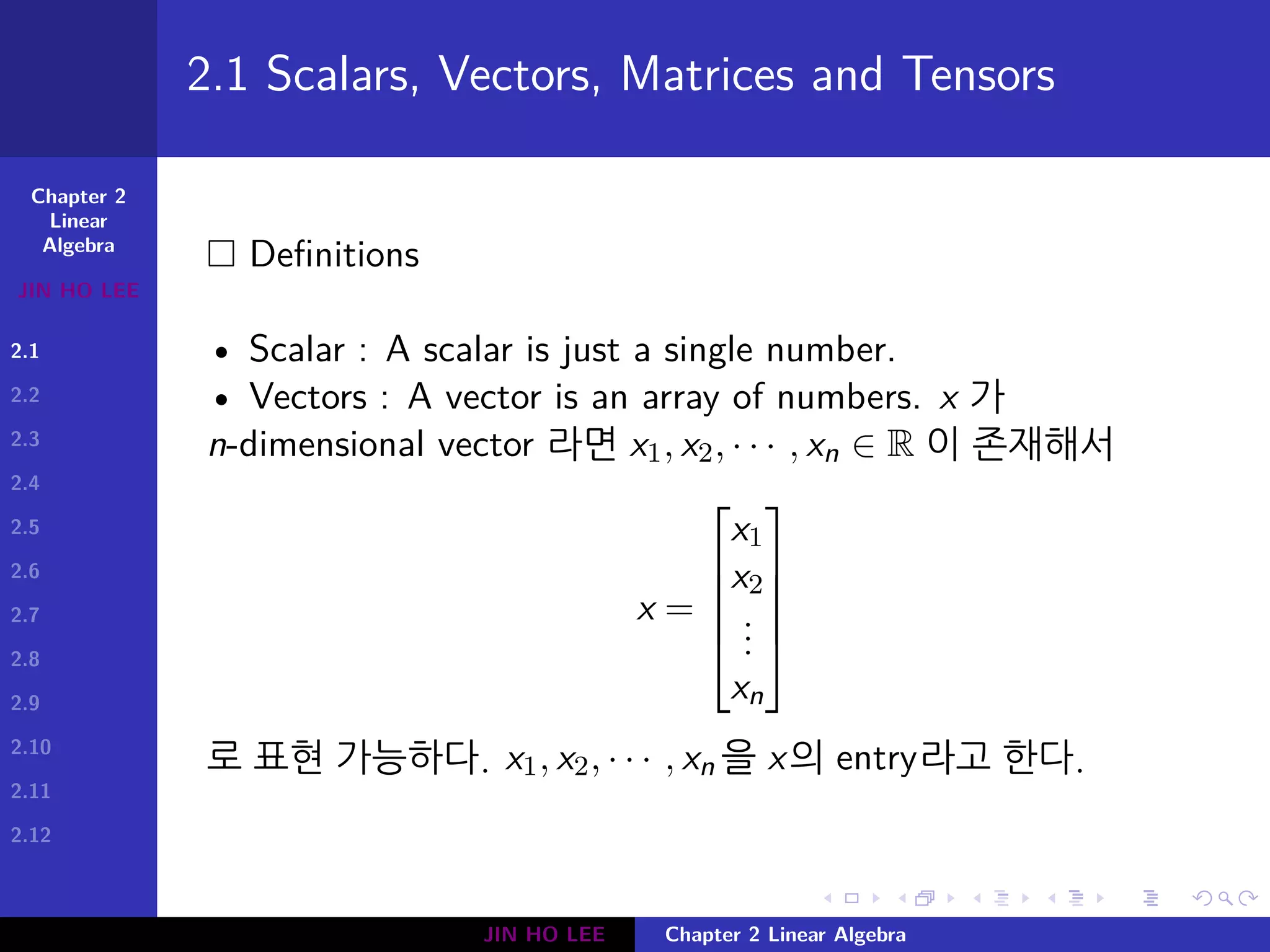
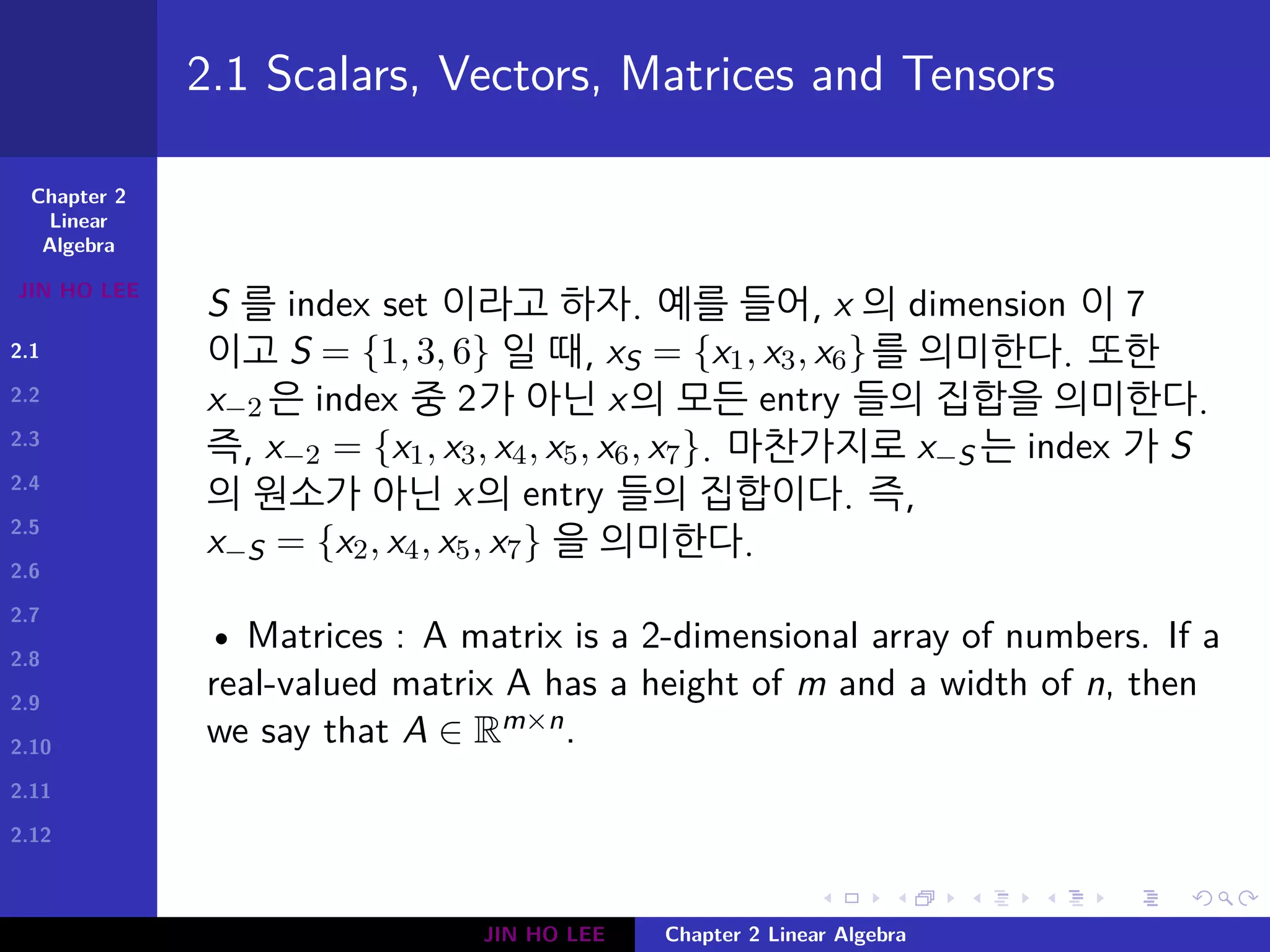
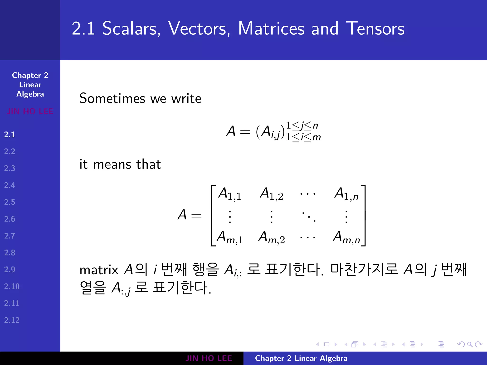
2.1 Scalars, Vectors, Matrices and Tensors
real valued function f 가 있을 때 matrix 에 적용할 수 있는데,
방법은 entry를 각각 f로 보내는 것이다. 예를 들어 f(x) = 2x
이고 A =
[
1 2
3 4
]
이면 f(A)i,j =
[
f(1) f(2)
f(3) f(4)
]
=
[
2 4
6 8
]
이다.
• Tensors : 3차원 이상의 숫자 배열을 tensor 라고 한다. A 의
(i, j, k) coordinate를 Ai,j,k 로 쓰자.
• Transpose : The transpose of a matrix AT is the mirror
image of the matrix across a diagonal line, called the main
diagonal, that is
(AT
)i,j = Aj,i.
JIN HO LEE Chapter 2 Linear Algebra

7. Chapter 2
Linear
Algebra
JIN HO LEE
2.1
2.2
2.3
2.4
2.5
2.6
2.7
2.8
2.9
2.10
2.11
2.12
.
.
.
.
.
.
.
.
.
.
.
.
.
.
.
.
.
.
.
.
.
.
.
.
.
.
.
.
.
.
.
.
.
.
.
.
.
.
.
.
2.2 Multiplying Matrices and Vectors
• matrix product : matrix A, B가 있을 때 matrix
multiplication C 는
Ci,j =
∑
k
Ai,kBk,j
로 정의된다. A 가 m × n matrix, B가 n × p matrix 이면 C는
m × p matrix 가 된다.
행렬의 크기(=행과 열의 갯수)가 같으면 element-wise
product(Hadamard product) A ⊙ B는 아래와 같의 정의된다:
(A ⊙ B)i,j = Ai,jBi,j.
JIN HO LEE Chapter 2 Linear Algebra

8. Chapter 2
Linear
Algebra
JIN HO LEE
2.1
2.2
2.3
2.4
2.5
2.6
2.7
2.8
2.9
2.10
2.11
2.12
.
.
.
.
.
.
.
.
.
.
.
.
.
.
.
.
.
.
.
.
.
.
.
.
.
.
.
.
.
.
.
.
.
.
.
.
.
.
.
.
2.2 Multiplying Matrices and Vectors
두 개의 n- dimensional vector x, y 의 dot product x · y는 아래와
같이 정의된다:
x · y = xT
y
= x1y1 + · · · + xnyn
JIN HO LEE Chapter 2 Linear Algebra

9. Chapter 2
Linear
Algebra
JIN HO LEE
2.1
2.2
2.3
2.4
2.5
2.6
2.7
2.8
2.9
2.10
2.11
2.12
.
.
.
.
.
.
.
.
.
.
.
.
.
.
.
.
.
.
.
.
.
.
.
.
.
.
.
.
.
.
.
.
.
.
.
.
.
.
.
.
2.3 Identity and Inverse Matrices
• Identity matrix : The n-dimensional identity matrix In
defined by
(In)i,j = δ(i, j)
where
δ(i, j) =
{
1 if i = j,
0 if i ̸= j,
• Matrix inverses : The matrix inverse of A is denoted as A−1,
and it is defined as the matrix such that
AA−1
= In.
JIN HO LEE Chapter 2 Linear Algebra

10. Chapter 2
Linear
Algebra
JIN HO LEE
2.1
2.2
2.3
2.4
2.5
2.6
2.7
2.8
2.9
2.10
2.11
2.12
.
.
.
.
.
.
.
.
.
.
.
.
.
.
.
.
.
.
.
.
.
.
.
.
.
.
.
.
.
.
.
.
.
.
.
.
.
.
.
.
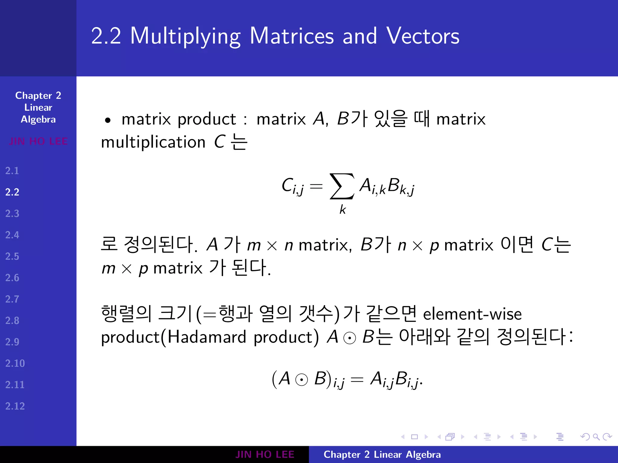
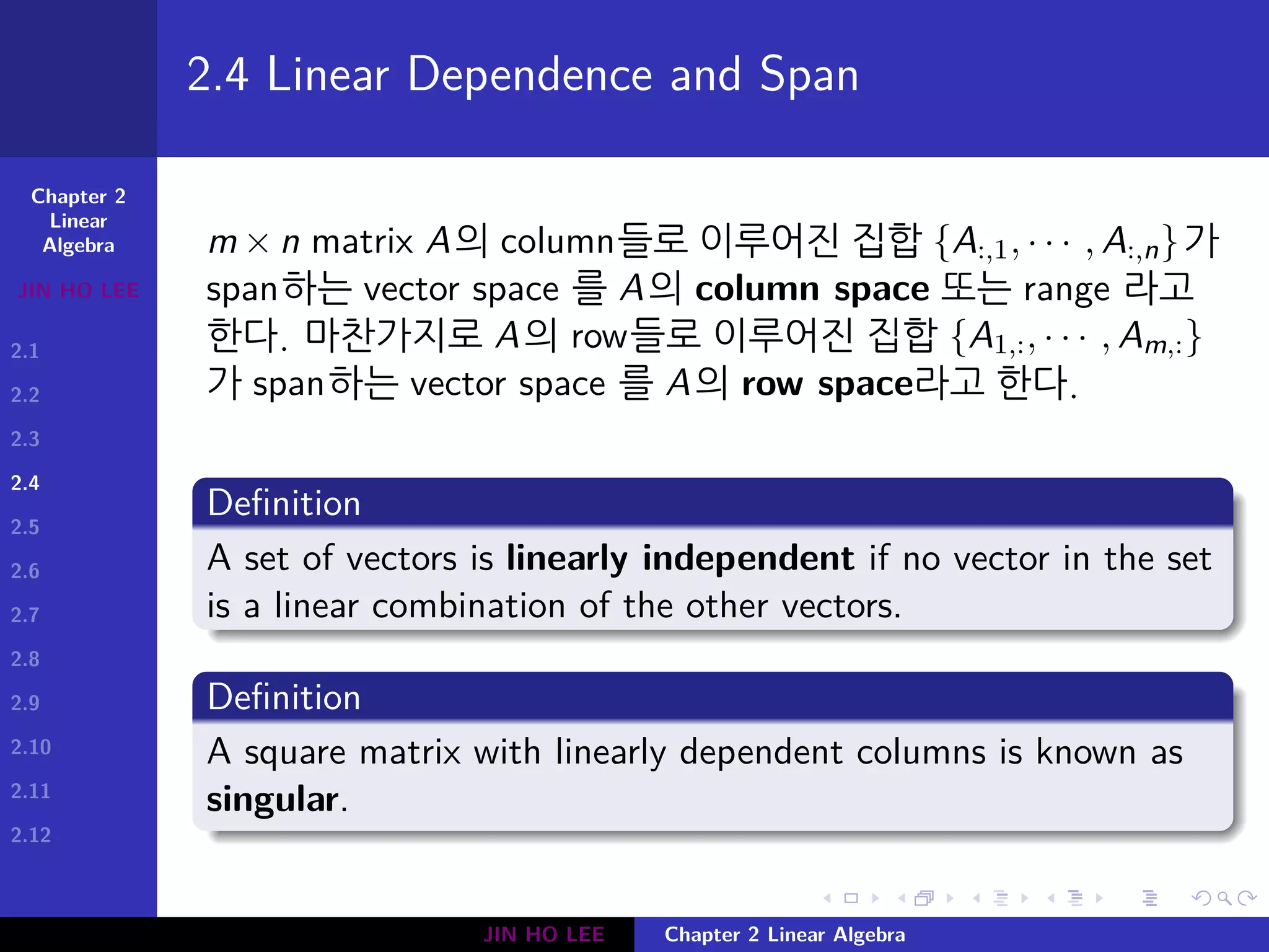
2.4 Linear Dependence and Span
scalar c1, · · · , cn 와 vector v(1), · · · , v(n) 가 있을 때
∑
i
civ(i)
= c1v(1)
+ · · · + ckv(n)
형태를 linear combination 이라고 한다.
vector 들의 집합 S = {v1, · · · , vn}가 있을 때, S가 span 하는
벡터공간 아래와 같이 정의된다:
{c1v1 + · · · + cnvn|c1, · · · , cn ∈ R}.
Example
v = [1, 2]T 일 때 {v1}가 span 하는 벡터공간은 아래와 같다:
{cv = [c, 2c]|c ∈ R}.
JIN HO LEE Chapter 2 Linear Algebra

11. Chapter 2
Linear
Algebra
JIN HO LEE
2.1
2.2
2.3
2.4
2.5
2.6
2.7
2.8
2.9
2.10
2.11
2.12
.
.
.
.
.
.
.
.
.
.
.
.
.
.
.
.
.
.
.
.
.
.
.
.
.
.
.
.
.
.
.
.
.
.
.
.
.
.
.
.
2.4 Linear Dependence and Span
m × n matrix A의 column들로 이루어진 집합 {A:,1, · · · , A:,n}가
span하는 vector space 를 A의 column space 또는 range 라고
한다. 마찬가지로 A의 row들로 이루어진 집합 {A1,:, · · · , Am,:}
가 span하는 vector space 를 A의 row space라고 한다.
Definition
A set of vectors is linearly independent if no vector in the set
is a linear combination of the other vectors.
Definition
A square matrix with linearly dependent columns is known as
singular.
JIN HO LEE Chapter 2 Linear Algebra

12. Chapter 2
Linear
Algebra
JIN HO LEE
2.1
2.2
2.3
2.4
2.5
2.6
2.7
2.8
2.9
2.10
2.11
2.12
.
.
.
.
.
.
.
.
.
.
.
.
.
.
.
.
.
.
.
.
.
.
.
.
.
.
.
.
.
.
.
.
.
.
.
.
.
.
.
.
2.5 Norms
Definition
A norm is any function f that satisfies the following properties:
• f(x) = 0 ⇒ x = 0
• f(x + y) ≤ f(x) + f(y) (the triangular inequality)
• ∀α ∈ R, f(αx) = |α|f(x)
JIN HO LEE Chapter 2 Linear Algebra

13. Chapter 2
Linear
Algebra
JIN HO LEE
2.1
2.2
2.3
2.4
2.5
2.6
2.7
2.8
2.9
2.10
2.11
2.12
.
.
.
.
.
.
.
.
.
.
.
.
.
.
.
.
.
.
.
.
.
.
.
.
.
.
.
.
.
.
.
.
.
.
.
.
.
.
.
.
2.5 Norms
Example
The Lp norm is given by
||x||p =
(
∑
i
|xi|p
)1
p
for all p ∈ R, p ≥ 1. The L2 norm is known as the Euclidean
norm.
Example
Given a vector x = (x1, · · · , xn), the max norm is defined by
||x||∞ = max
i
|xi|.
JIN HO LEE Chapter 2 Linear Algebra

14. Chapter 2
Linear
Algebra
JIN HO LEE
2.1
2.2
2.3
2.4
2.5
2.6
2.7
2.8
2.9
2.10
2.11
2.12
.
.
.
.
.
.
.
.
.
.
.
.
.
.
.
.
.
.
.
.
.
.
.
.
.
.
.
.
.
.
.
.
.
.
.
.
.
.
.
.
2.5 Norms
Example
Given a matrix A, the Frobenius norm is defined by
||A||F =
√∑
i,j
A2
i,j.
JIN HO LEE Chapter 2 Linear Algebra

15. Chapter 2
Linear
Algebra
JIN HO LEE
2.1
2.2
2.3
2.4
2.5
2.6
2.7
2.8
2.9
2.10
2.11
2.12
.
.
.
.
.
.
.
.
.
.
.
.
.
.
.
.
.
.
.
.
.
.
.
.
.
.
.
.
.
.
.
.
.
.
.
.
.
.
.
.
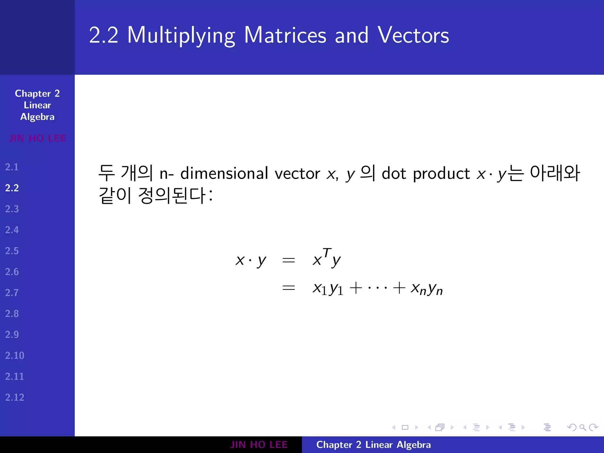
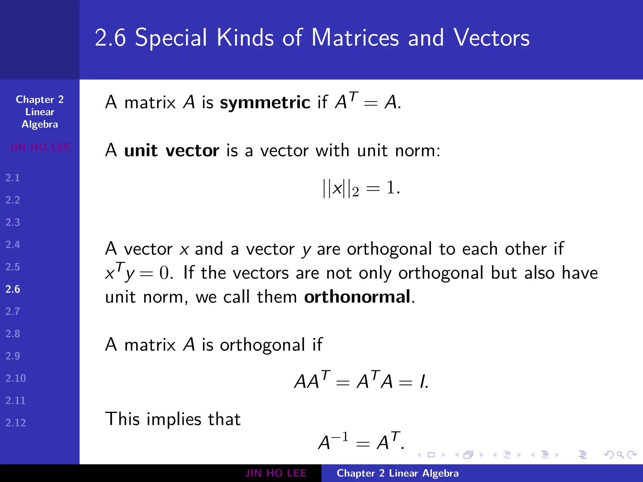
2.6 Special Kinds of Matrices and Vectors
Definition
A matrix D is diagonal if Di,j = 0 for i ̸= j.
Given a vector v = (v1, · · · , vn), we write diag(v) to denote a
square diagonal matrix whose diagonal entries are given by the
entries of the vector v. For a vector v = (1, 2), we have
diag(v) =
[
1 0
0 2
]
It is clear that diag(v)x = v ⊙ x for any vector x. If vi ̸= 0 for
any i = 1, · · · , n, we denote
diag(v)−1
= diag([1/v1, · · · , 1/vn]T
).
JIN HO LEE Chapter 2 Linear Algebra

16. Chapter 2
Linear
Algebra
JIN HO LEE
2.1
2.2
2.3
2.4
2.5
2.6
2.7
2.8
2.9
2.10
2.11
2.12
.
.
.
.
.
.
.
.
.
.
.
.
.
.
.
.
.
.
.
.
.
.
.
.
.
.
.
.
.
.
.
.
.
.
.
.
.
.
.
.
2.6 Special Kinds of Matrices and Vectors
A matrix A is symmetric if AT = A.
A unit vector is a vector with unit norm:
||x||2 = 1.
A vector x and a vector y are orthogonal to each other if
xTy = 0. If the vectors are not only orthogonal but also have
unit norm, we call them orthonormal.
A matrix A is orthogonal if
AAT
= AT
A = I.
This implies that
A−1
= AT
.
JIN HO LEE Chapter 2 Linear Algebra

17. Chapter 2
Linear
Algebra
JIN HO LEE
2.1
2.2
2.3
2.4
2.5
2.6
2.7
2.8
2.9
2.10
2.11
2.12
.
.
.
.
.
.
.
.
.
.
.
.
.
.
.
.
.
.
.
.
.
.
.
.
.
.
.
.
.
.
.
.
.
.
.
.
.
.
.
.
2.7 Eigendecomposition
Definition
An eigenvector of a square matrix A is a non-zero vector v
such that multiplication by A alters only the scale of v:
Av = λv.
The scalar λ is known as the eigenvalue corresponding to this
eigenvector
eigenvector에 scalar product 를 해도 eigenvector 가 되므로
우리는 항상 unit eigenvector만 다루기로 하자.
JIN HO LEE Chapter 2 Linear Algebra

18. Chapter 2
Linear
Algebra
JIN HO LEE
2.1
2.2
2.3
2.4
2.5
2.6
2.7
2.8
2.9
2.10
2.11
2.12
.
.
.
.
.
.
.
.
.
.
.
.
.
.
.
.
.
.
.
.
.
.
.
.
.
.
.
.
.
.
.
.
.
.
.
.
.
.
.
.
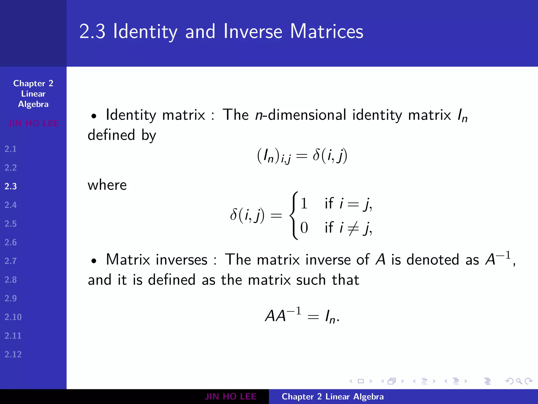
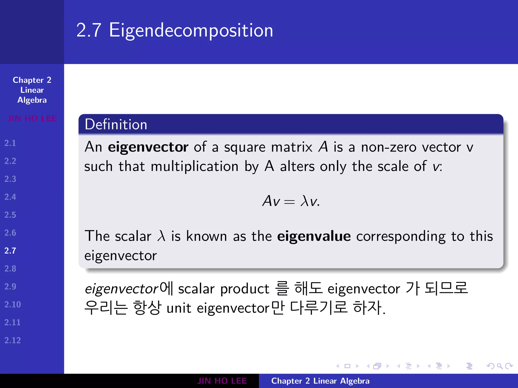
2.7 Eigendecomposition
Suppose that a matrix A has n linearly independent
eigenvectors, {v(1), · · · , v(n)}, with corresponding eigenvalues
{λ1, ..., λn}. We may concatenate all of the eigenvectors to
form a matrix V with one eigenvector per column:
V = [v(1), · · · , v(n)]. Likewise, we can concatenate the
eigenvalues to form a vector λ = [λ1, · · · , λn].
The eigendecomposition of A is then given by
A = V diag(λ) V−1
.
JIN HO LEE Chapter 2 Linear Algebra

19. Chapter 2
Linear
Algebra
JIN HO LEE
2.1
2.2
2.3
2.4
2.5
2.6
2.7
2.8
2.9
2.10
2.11
2.12
.
.
.
.
.
.
.
.
.
.
.
.
.
.
.
.
.
.
.
.
.
.
.
.
.
.
.
.
.
.
.
.
.
.
.
.
.
.
.
.
2.8 Singular Value Decomposition(SVD)
A matrix A can be broken into product of 3 matrices as follow:
Am×n = Um×mΛm×nVT
n×n
where
• UTU = I, VTV = I,
• columns of U are consists of orthonormal eigenvectors of
AAT, (i.e. UTU = I)
• columns of V are consists of orthonormal eigenvectors of
ATA, (i.e. VTV = I)
• S is a diagonal matrix containing square roots of eigenvalues
from U or V in descending order.
JIN HO LEE Chapter 2 Linear Algebra

20. Chapter 2
Linear
Algebra
JIN HO LEE
2.1
2.2
2.3
2.4
2.5
2.6
2.7
2.8
2.9
2.10
2.11
2.12
.
.
.
.
.
.
.
.
.
.
.
.
.
.
.
.
.
.
.
.
.
.
.
.
.
.
.
.
.
.
.
.
.
.
.
.
.
.
.
.
2.8 Singular Value Decomposition(SVD)
For a symmatric matrix A, we can write A = UΛUT since
ATA = AAT. Then we have
AT
A = UΛUT
UΛUT
= UΛ2
UT
= Udiag(λ)UT
.
This implies that Λ2 = diag(λ).
A matrix whose eigenvalues are all positive is called positive
definite. A matrix whose eigenvalues are all positive or
zero-valued is called positive semidefinite. Positive
semidefinite matrices are interesting because they guarantee
that ∀x, xTAx ≥ 0. Positive definite matrices additionally
guarantee that xTAx = 0 ⇒ x = 0.
JIN HO LEE Chapter 2 Linear Algebra

21. Chapter 2
Linear
Algebra
JIN HO LEE
2.1
2.2
2.3
2.4
2.5
2.6
2.7
2.8
2.9
2.10
2.11
2.12
.
.
.
.
.
.
.
.
.
.
.
.
.
.
.
.
.
.
.
.
.
.
.
.
.
.
.
.
.
.
.
.
.
.
.
.
.
.
.
.
2.9 The Moore-Penrose Pseudoinverse
이번 절에서는 nonsquare matrix 의 matrix inversion에 대해
알아보자.
Definition
The pseudoinverse of A is defined as a matrix
A+
= lim
α↘0
(AT
A + αI)−1
AT
.
여기서 lim
α↘0
는 α가 양수인 상태에서 0으로 가까이 간다는
의미이다. 다른 책에서는 lim
δ→0
(ATA + δ2I)−1AT 로 표현했는데
두 개는 같은 의미이다. 자세한 내용은 아래 파일을 참고!
http://www.math.ucla.edu/~laub/33a.2.12s/
mppseudoinverse.pdf
JIN HO LEE Chapter 2 Linear Algebra

22. Chapter 2
Linear
Algebra
JIN HO LEE
2.1
2.2
2.3
2.4
2.5
2.6
2.7
2.8
2.9
2.10
2.11
2.12
.
.
.
.
.
.
.
.
.
.
.
.
.
.
.
.
.
.
.
.
.
.
.
.
.
.
.
.
.
.
.
.
.
.
.
.
.
.
.
.
2.9 The Moore-Penrose Pseudoinverse
matrix A 의 SVD가 A = UDVT 일 때, psedoinverse는 아래와
같다:
A+
= VD+
UT
.
JIN HO LEE Chapter 2 Linear Algebra

23. Chapter 2
Linear
Algebra
JIN HO LEE
2.1
2.2
2.3
2.4
2.5
2.6
2.7
2.8
2.9
2.10
2.11
2.12
.
.
.
.
.
.
.
.
.
.
.
.
.
.
.
.
.
.
.
.
.
.
.
.
.
.
.
.
.
.
.
.
.
.
.
.
.
.
.
.
2.10 The Trace Operator
Definition
The trace operator gives the sum of all of the diagonal entries
of a matrix:
Tr(A) =
∑
i
Ai,i.
Lemma
1. ||A|||F =
√
Tr(AAT).
2. Tr(A) = Tr(AT).
3-1. Tr(ABC) = Tr(CAB) = Tr(BCA).
3-2. More generaly, Tr(
∏n
i=1 F(i)) = Tr(F(n)
∏n−1
i=1 F(i)).
4. For, A ∈ Rm×n, B ∈ Rn×m, Tr(AB) = Tr(BA).
JIN HO LEE Chapter 2 Linear Algebra

24. Chapter 2
Linear
Algebra
JIN HO LEE
2.1
2.2
2.3
2.4
2.5
2.6
2.7
2.8
2.9
2.10
2.11
2.12
.
.
.
.
.
.
.
.
.
.
.
.
.
.
.
.
.
.
.
.
.
.
.
.
.
.
.
.
.
.
.
.
.
.
.
.
.
.
.
.
2.11 The Determinant
The determinant of a square matrix, denoted det(A), is a
function mapping matrices to real scalars. The determinant is
equal to the product of all the eigenvalues of the matrix. The
absolute value of the determinant can be thought of as a
measure of how much multiplication by the matrix expands or
contracts space.
자세한 내용은 wiki의 determinant, cofactor expansion 을
참고하자!
JIN HO LEE Chapter 2 Linear Algebra

25. Chapter 2
Linear
Algebra
JIN HO LEE
2.1
2.2
2.3
2.4
2.5
2.6
2.7
2.8
2.9
2.10
2.11
2.12
.
.
.
.
.
.
.
.
.
.
.
.
.
.
.
.
.
.
.
.
.
.
.
.
.
.
.
.
.
.
.
.
.
.
.
.
.
.
.
.
2.12 Example: Principal Components Analysis
n-dimensional points {x(1), · · · , x(m)} 이 있다고 하자. 이번
절에서는 lossy comprehension에 대해 알아보자. 여기서 lossy
comprehension 이란, point 갯수는 줄이는데 precision은 조금만
낮추는 것을 의미한다.(즉, 데이터 수는 줄이지만 정보는 조금만
잃는 상태를 원한다)
한 가지 방법은 l n에 대해서 f : Rn → Rl 을 이용하여
encoding 하는 것이다. 각각의 i에 대해 f(x(i)) = c(i) 로 차원을
축소하고, decoder g : Rl → Rn 을 사용하여 다시 차원을
복귀시켜 원래의 값과 비슷하게 만드는것이 목표이다. 앞으로는
x ≈ g(f(x)) 로 만든 다음 두 값의 차이를 loss function 으로 놓고
그것을 minimize 하려고 한다.
JIN HO LEE Chapter 2 Linear Algebra

26. Chapter 2
Linear
Algebra
JIN HO LEE
2.1
2.2
2.3
2.4
2.5
2.6
2.7
2.8
2.9
2.10
2.11
2.12
.
.
.
.
.
.
.
.
.
.
.
.
.
.
.
.
.
.
.
.
.
.
.
.
.
.
.
.
.
.
.
.
.
.
.
.
.
.
.
.
2.12 Example: Principal Components Analysis
g 는 (n × l)− matrix D로 놓을 수 있다. 우리는 D를 orthonomal
이라고 가정하자.
f(x) = c 일 때, 우리의 목표는
c∗
= argmin
c
||x − g(c)||2
2
를 찾는 것이다. 이제 수식을 풀어보자.
||x − g(c)||2
2 = (x − g(c))T
(x − g(c))
= xT
x − xT
g(c) − g(c)T
x + g(x)T
g(c)
= xT
x − 2xT
g(c) + g(c)T
g(c) (1)
여기서 x, g(c)T ∈ Rn 이므로 matrix multiplication xTg(c)와
g(c)Tx 모두 실수이므로 xTg(c) = g(c)Tx 이다.
JIN HO LEE Chapter 2 Linear Algebra

27. Chapter 2
Linear
Algebra
JIN HO LEE
2.1
2.2
2.3
2.4
2.5
2.6
2.7
2.8
2.9
2.10
2.11
2.12
.
.
.
.
.
.
.
.
.
.
.
.
.
.
.
.
.
.
.
.
.
.
.
.
.
.
.
.
.
.
.
.
.
.
.
.
.
.
.
.
2.12 Example: Principal Components Analysis
수식 (1)에서 xTx는 x에 대한 함수이므로 argmin
c
에 의해
영향을 받지 않는다. 또한 g는 orthonormal matrix D라고
했으므로 DTD = Il 을 이용하여, (1)을 아래와 같이 쓸 수 있다.
c∗
= argmin
c
−2xT
Dc + cT
DT
Dc
= argmin
c
−2xT
Dc + cT
c (2)
수식 (2)의 함수 h(c) = −2xTDc + cTc의 minimum을 체크하기
위해 미분값이 0이 되는 조건을 체크해보자.
∇c(−2xT
Dc + cT
c) = −2DxT
+ 2c = 0
c = DT
x.
따라서 f(x) = DTx 이다.
JIN HO LEE Chapter 2 Linear Algebra

28. Chapter 2
Linear
Algebra
JIN HO LEE
2.1
2.2
2.3
2.4
2.5
2.6
2.7
2.8
2.9
2.10
2.11
2.12
.
.
.
.
.
.
.
.
.
.
.
.
.
.
.
.
.
.
.
.
.
.
.
.
.
.
.
.
.
.
.
.
.
.
.
.
.
.
.
.
2.12 Example: Principal Components Analysis
We define the PCA representation operation:
r(x) = g(f(x)) = DDT
x.
이제 최적의 D 를 찾아보자. D는 reconstruction error 가 작아야
하므로 아래의 식을 만족시키는 D∗ 를 찾으면 된다.
D∗
= argmin
D
√∑
i,j
(x
(i)
j − r(x
(i)
j ))2 subject to DT
D = Il
앞에서 D는 orthonormal 이라고 가정했기때문에 DTD = Il
조건이 들어갔다.
JIN HO LEE Chapter 2 Linear Algebra

29. Chapter 2
Linear
Algebra
JIN HO LEE
2.1
2.2
2.3
2.4
2.5
2.6
2.7
2.8
2.9
2.10
2.11
2.12
.
.
.
.
.
.
.
.
.
.
.
.
.
.
.
.
.
.
.
.
.
.
.
.
.
.
.
.
.
.
.
.
.
.
.
.
.
.
.
.
2.12 Example: Principal Components Analysis
먼저 l = 1인 경우에 대해 알아보자.
d∗
= argmin
d
∑
i
||x(i)
− ddT
x(i)
||2
2 subject to ||d||2 = 1. (3)
l = 1이므로 d = D는 (n × l) = (n × 1)− matrix 이므로
n-dimensional vector이다. 즉, matrix multiplication dTx(i) 의
결과는 실수이므로 ddTx(i) 는 d라는 vector에 dTx(i) 라는 scalar
를 scalar multiplication 한 것이어서 ddTx(i) = dTx(i)d 를 얻을
수 있다. 그리고 scalar 는 자기 자신의 transpose 이므로
(dTx(i))T = x(i)T
d 이다.
JIN HO LEE Chapter 2 Linear Algebra

30. Chapter 2
Linear
Algebra
JIN HO LEE
2.1
2.2
2.3
2.4
2.5
2.6
2.7
2.8
2.9
2.10
2.11
2.12
.
.
.
.
.
.
.
.
.
.
.
.
.
.
.
.
.
.
.
.
.
.
.
.
.
.
.
.
.
.
.
.
.
.
.
.
.
.
.
.
2.12 Example: Principal Components Analysis
Thus we have
d∗
= argmin
d
∑
i
||x(i)
− dT
x(i)
d||2
2 subject to ||d||2 = 1
= argmin
d
∑
i
||x(i)
− x(i)T
dd||2
2 subject to ||d||2 = 1
Let X ∈ Rm×n and Xi,: = x(i)T
∈ Rn. It is clear that
||X||F =
n∑
i=1
||x(i)T
||F. (4)
JIN HO LEE Chapter 2 Linear Algebra

31. Chapter 2
Linear
Algebra
JIN HO LEE
2.1
2.2
2.3
2.4
2.5
2.6
2.7
2.8
2.9
2.10
2.11
2.12
.
.
.
.
.
.
.
.
.
.
.
.
.
.
.
.
.
.
.
.
.
.
.
.
.
.
.
.
.
.
.
.
.
.
.
.
.
.
.
.
2.12 Example: Principal Components Analysis
(4)와 trace의 성질 Tr(A) = Tr(AT)을 이용하여 (3)은 아래와
같이 변형할 수 있다:
d∗
= argmin
d
∑
i
||X − ddT
x(i)
||2
2 subject to ||d||2 = 1
because (x(i)T
− ddTx(i)T
)T = x(i) − x(i)ddT. We can simplify
the Frobenious norm as follows:
argmin
d
||X − XddT||2
F
= argmin
d
Tr((X − XddT)T(X − XddT))
= argmin
d
(−Tr(XTXddT) − Tr(ddTXTX) + Tr(ddTXTXddT))
JIN HO LEE Chapter 2 Linear Algebra

32. Chapter 2
Linear
Algebra
JIN HO LEE
2.1
2.2
2.3
2.4
2.5
2.6
2.7
2.8
2.9
2.10
2.11
2.12
.
.
.
.
.
.
.
.
.
.
.
.
.
.
.
.
.
.
.
.
.
.
.
.
.
.
.
.
.
.
.
.
.
.
.
.
.
.
.
.
2.12 Example: Principal Components Analysis
(XTXddT)T = ddTXTX 이므로 (2.52)를 이용하여 위의 식을
아래와 같이 변형할 수 있다:
= argmin
d
(−2Tr(XT
XddT
) + Tr(XT
XddT
ddT
)).
이제 constraint dTd = 1 을 이용해서 다시 정리해보자.
argmin
d
(−2Tr(XT
XddT
)+Tr(XT
XddT
ddT
)) subject to dT
d = 1
= argmin
d
(−2Tr(XT
XddT
) + Tr(XT
XddT
) subject to dT
d = 1
= argmin
d
(−Tr(XT
XddT
)) subject to dT
d = 1
JIN HO LEE Chapter 2 Linear Algebra

33. Chapter 2
Linear
Algebra
JIN HO LEE
2.1
2.2
2.3
2.4
2.5
2.6
2.7
2.8
2.9
2.10
2.11
2.12
.
.
.
.
.
.
.
.
.
.
.
.
.
.
.
.
.
.
.
.
.
.
.
.
.
.
.
.
.
.
.
.
.
.
.
.
.
.
.
.
2.12 Example: Principal Components Analysis
= argmax
d
Tr(XT
XddT
) subject to dT
d = 1
식 (2.52)를 이용해서 아래의 결과를 얻을 수 있다:
= argmax
d
Tr(dT
XT
Xd) subject to dT
d = 1
이 문제는 eigendecomposition 을 이용하여 풀 수 있다. (d 는
XTX의 가장 큰 eigenvector의 eigenvector).
l 1의 경우에 행렬 D는 l largest eigenvalue의 eigenvector
들이다.
JIN HO LEE Chapter 2 Linear Algebra