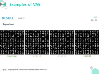
In this chapter,we will discuss about
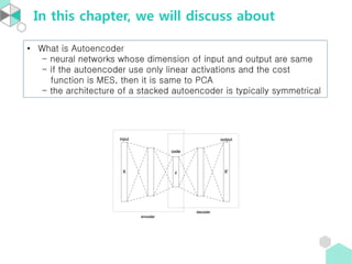
• What is Autoencoder
- neural networks whose dimension of input and output are same
- if the autoencoder use only linear activations and the cost
function is MES, then it is same to PCA
- the architecture of a stacked autoencoder is typically symmetrical
Introduction
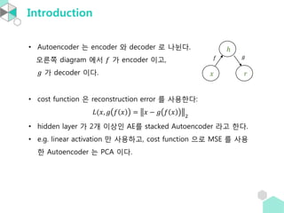
• Autoencoder 는encoder 와 decoder 로 나뉜다.
오른쪽 diagram 에서 𝑓 가 encoder 이고,
𝑔 가 decoder 이다.
• cost function 은 reconstruction error 를 사용한다:
𝐿(𝑥, 𝑔 𝑓 𝑥 = 𝑥 − 𝑔 𝑓 𝑥 2
• hidden layer 가 2개 이상인 AE를 stacked Autoencoder 라고 한다.
• e.g. linear activation 만 사용하고, cost function 으로 MSE 를 사용
한 Autoencoder 는 PCA 이다.
𝑥
ℎ
𝑟
𝑓 𝑔
6.
Introduction
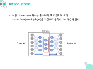
• 보통 hiddenlayer 개수는 홀수이며 AE의 정의에 의해
center layer(=coding layer)를 기준으로 양쪽의 unit 개수가 같다.
Coding layer
Encoder Decoder
7.
Introduction
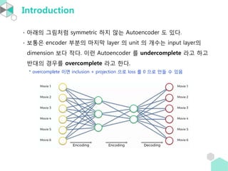
∙ 아래의 그림처럼symmetric 하지 않는 Autoencoder 도 있다.
∙ 보통은 encoder 부분의 마지막 layer 의 unit 의 개수는 input layer의
dimension 보다 작다. 이런 Autoencoder 를 undercomplete 라고 하고
반대의 경우를 overcomplete 라고 한다.
* overcomplete 이면 inclusion + projection 으로 loss 를 0 으로 만들 수 있음
8.
Cost function
• [VLBM,p.2] An autoencoder takes an input vector 𝑥 ∈ 0,1 𝑑
, and first
maps it to a hidden representation y ∈ 0,1 𝑑′
through a deterministic
mapping 𝑦 = 𝑓𝜃 𝑥 = 𝑠(𝑊𝑥 + 𝑏), parameterized by 𝜃 = {𝑊, 𝑏}.
𝑊 is a 𝑑 × 𝑑′
weight matrix and 𝒃 is a bias vector. The resulting latent
representation 𝑦 is then mapped back to a “reconstructed” vector
z ∈ 0,1 𝑑 in input space 𝑧 = 𝑔 𝜃′ 𝑦 = 𝑠 𝑊′ 𝑦 + 𝑏′ with 𝜃′ = {𝑊′, 𝑏′}.
The weight matrix 𝑊′ of the reverse mapping may optionally be
constrained by 𝑊′ = 𝑊 𝑇, in which case the autoencoder is said to
have tied weights.
• The parameters of this model are optimized to minimize
the average reconstruction error:
𝜃∗
, 𝜃′∗
= arg min
𝜃,𝜃′
1
𝑛
𝑖=1
𝑛
𝐿(𝑥 𝑖
, 𝑧 𝑖
)
= arg min
𝜃,𝜃′
1
𝑛 𝑖=1
𝑛
𝐿(𝑥 𝑖
, 𝑔 𝜃′(𝑓𝜃 𝑥 𝑖
) (1)
where 𝐿 𝑥 − 𝑧 = 𝑥 − 𝑧 2.
9.
Cost function
• [VLBM,p.2]An alternative loss, suggested by the interpretation of 𝑥
and 𝑧 as either bit vectors or vectors of bit probabilities (Bernoullis) is
the reconstruction cross-entropy:
𝐿 𝐻 𝑥, 𝑧 = 𝐻(𝐵𝑥||𝐵𝑧)
= − 𝑘=1
𝑑
[𝑥 𝑘 log 𝑧 𝑘 + log 1 − 𝑥 𝑘 log(1 − 𝑧 𝑘)]
where 𝐵𝜇 𝑥 = (𝐵𝜇1
𝑥 , ⋯ , 𝐵𝜇 𝑑
𝑥 ) is a Bernoulli distribution.
• [VLBM,p.2] Equation (1) with 𝐿 = 𝐿 𝐻 can be written
𝜃∗, 𝜃′∗ = arg min
𝜃,𝜃′
𝐸 𝑞0 [𝐿 𝐻(𝑋, 𝑔 𝜃′(𝑓𝜃 𝑋 ))]
where 𝑞0(𝑋) denotes the empirical distribution associated to our 𝑛
training inputs.
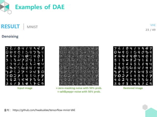
Denoising Autoencoders
• [VLBM,p.3]corrupted input 를 넣어 repaired input 을 찾는 training
을 한다. 좀 더 정확하게 말하면 input data의 dimension 이 𝑑 라고
할 때 ‘desired proportion 𝜈 of destruction’ 을 정하여 𝜈𝑑 만큼의
input 을 0 으로 수정하는 방식으로 destruction 한다. 여기서 𝜈𝑑 개
components 는 random 으로 정한다. 이후 reconstruction error 를
체크하여 destruction 전의 input 으로 복구하는 cost function
이용하여 학습을 하는 Autoencoder 가 Denoising Autoencoder 이다.
여기서 𝑥 에서 destroyed version 인 𝑥 를 얻는 과정은 stochastic
mapping 𝑥 ~ 𝑞 𝐷( 𝑥|x) 를 따른다.
12.
Denoising Autoencoders
• [VLBM,p.3]Let us define the joint distribution
𝑞0
𝑋, 𝑋, 𝑌 = 𝑞0
𝑋 𝑞 𝐷 𝑋 𝑋 𝛿𝑓 𝜃 𝑋
(𝑌))
where 𝛿 𝑢(𝑣) is the Kronecker delta. Thus 𝑌 is a deterministic
function of 𝑋. 𝑞0(𝑋, 𝑋, 𝑌) is parameterized by 𝜃. The objective
function minimized by stochastic gradient descent becomes:
𝑎𝑟𝑔 𝑚𝑖𝑛
𝜃,𝜃′
𝐸 𝑞0 𝑥, 𝑥 [𝐿 𝐻(𝑥, 𝑔 𝜃′(𝑓𝜃( 𝑥))])
Corrupted 𝑥 를 입력하고 𝑥 를 찾는 방법으로 학습!
13.
Other Autoencoders
• [DLbook, 14.2.1] A sparse autoencoder is simply an autoencoder
whose training criterion involves a sparsity penalty Ω ℎ on the
code layer h, in addition to the reconstruction error:
𝐿(𝑥, 𝑔 𝑓 𝑥 ) + Ω(ℎ),
where 𝑔 ℎ is the decoder output and typically we have ℎ = 𝑓(𝑥),
the encoder output.
• [DL book, 14.2.3] Another strategy for regularizing an autoencoder
is to use a penalty Ω as in sparse autoencoders,
𝐿 𝑥, 𝑔 𝑓 𝑥 ) + Ω(ℎ, 𝑥 ,
but with a different form of Ω:
Ω ℎ, 𝑥 = 𝜆
𝑖
𝛻𝑥ℎ𝑖
2
Reference
• Reference. Auto-EncodingVariational Bayes, Diederik P Kingma,
Max Welling, 2013
• [논문의 가정] We will restrict ourselves here to the common case
where we have an i.i.d. dataset with latent variables per datapoint,
and where we like to perform maximum likelihood (ML) or
maximum a posteriori (MAP) inference on the (global) parameters,
and variational inference on the latent variables.
16.
Definition
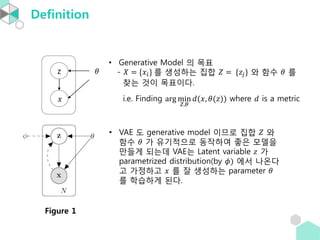
• Generative Model의 목표
- 𝑋 = {𝑥𝑖} 를 생성하는 집합 𝑍 = {𝑧𝑗} 와 함수 𝜃 를
찾는 것이 목표이다.
i.e. Finding arg min
𝑍,𝜃
𝑑(𝑥, 𝜃(𝑧)) where 𝑑 is a metric
• VAE 도 generative model 이므로 집합 𝑍 와
함수 𝜃 가 유기적으로 동작하여 좋은 모델을
만들게 되는데 VAE는 Latent variable 𝑧 가
parametrized distribution(by 𝜙) 에서 나온다
고 가정하고 𝑥 를 잘 생성하는 parameter 𝜃
를 학습하게 된다.
Figure 1
z
𝑥
𝜃
17.
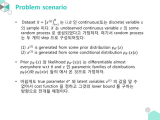
Problem scenario
• Dataset𝑋 = 𝑥 𝑖
𝑖=1
𝑁
는 i.i.d 인 continuous(또는 discrete) variable 𝑥
의 sample 이다. 𝑋 는 unobserved continuous variable 𝑧 의 some
random process 로 생성되었다고 가정하자. 여기서 random process
는 두 개의 step 으로 구성되어있다:
(1) 𝑧(𝑖)
is generated from some prior distribution 𝑝 𝜃∗(𝑧)
(2) 𝑥(𝑖)
is generated from some conditional distribution 𝑝 𝜃∗(𝑥|𝑧)
• Prior 𝑝 𝜃∗ 𝑧 와 likelihood 𝑝 𝜃∗(𝑥|𝑧) 는 differentiable almost
everywhere w.r.t 𝜃 and 𝑧 인 parametric families of distributions
𝑝 𝜃(𝑧)와 𝑝 𝜃(𝑥|𝑧) 들의 에서 온 것으로 가정하자.
• 아쉽게도 true parameter 𝜃∗
와 latent variables 𝑧(𝑖)
의 값을 알 수
없어서 cost function 을 정하고 그것의 lower bound 를 구하는
방향으로 전개될 예정이다.
18.
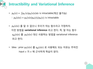
Intractibility and VariationalInference
• 𝑝 𝜃 𝑥 = 𝑝 𝜃 𝑥 𝑝 𝜃 𝑥 𝑧 𝑑𝑧 is intractable(계산 불가능)
∵ 𝑝 𝜃 𝑧 𝑥 = 𝑝 𝜃 𝑥 𝑧 𝑝 𝜃(𝑧)/𝑝 𝜃(𝑥) is intractable
• 𝑝 𝜃 𝑧 𝑥 를 알 수 없으니 우리가 아는 함수라고 가정하자.
이런 방법을 variational inference 라고 한다. 즉, 잘 아는 함수
𝑞 𝜙(𝑧|𝑥) 를 𝑝 𝜃 𝑧 𝑥 대신 사용하는 방법을 variational inference
라고 한다.
• Idea : prior 𝑝 𝜃 𝑧 𝑥 를 𝑞 𝜙(𝑧|𝑥) 로 사용해도 되는 이유는 주어진
input 𝑧 가 𝑥 에 근사하게 학습이 된다.
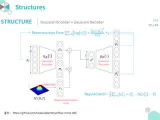
Reconstruction error 학습방법
• 𝐸 𝑞 𝜙 𝑧 𝑥 [log 𝑝 𝜃(𝑥|𝑧)]는 sampling 을 통해 Monte-carlo estimation 한다.
즉, 𝑥𝑖 ∈ X 마다 𝑧 𝑖,1
, ⋯ , 𝑧 𝑖 𝐿 를 sampling 하여 log likelihood 의 mean으로
근사시킨다. 보통 𝐿 = 1 을 많이 사용한다.
𝐸 𝑞 𝜙 𝑧 𝑥 [log 𝑝 𝜃(𝑥|𝑧)] ∼
1
𝐿
Σ𝑙=1
𝐿
log(𝑝 𝜃 𝑥𝑖 𝑧 𝑖,𝑙 )
• 이렇게 sampling 을 하면 backpropagation 을 할 수 없다. 그래서 사용
되는 방법이 reparametrization trick 이다.
𝑞 𝜙 𝑥 𝑧 𝑝 𝜃 𝑥 𝑧
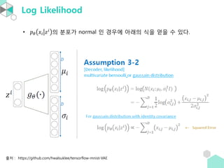
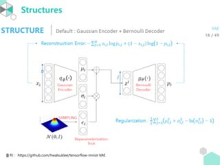
Log Likelihood
• 앞에서reconstruction error 를 계산할 때 하나씩 sampling 을 하면
𝐸 𝑞 𝜙 𝑧 𝑥 [log 𝑝 𝜃(𝑥|𝑧)] ∼
1
𝐿
Σ𝑙=1
𝐿
log 𝑝 𝜃 𝑥𝑖 𝑧 𝑖,𝑙
= log(𝑝 𝜃(𝑥𝑖|𝑧 𝑖
)
가 된다. 여기서 𝑝 𝜃 𝑥𝑖 𝑧 𝑖
의 분포가 Bernoulli 인 경우에 아래의 식을
얻을 수 있다.
출처 : https://github.com/hwalsuklee/tensorflow-mnist-VAE
25.
Log Likelihood
• 𝑝𝜃 𝑥𝑖 𝑧 𝑖 의 분포가 normal 인 경우에 아래의 식을 얻을 수 있다.
출처 : https://github.com/hwalsuklee/tensorflow-mnist-VAE


![Cost function
• [VLBM, p.2] An autoencoder takes an input vector 𝑥 ∈ 0,1 𝑑
, and first
maps it to a hidden representation y ∈ 0,1 𝑑′
through a deterministic
mapping 𝑦 = 𝑓𝜃 𝑥 = 𝑠(𝑊𝑥 + 𝑏), parameterized by 𝜃 = {𝑊, 𝑏}.
𝑊 is a 𝑑 × 𝑑′
weight matrix and 𝒃 is a bias vector. The resulting latent
representation 𝑦 is then mapped back to a “reconstructed” vector
z ∈ 0,1 𝑑 in input space 𝑧 = 𝑔 𝜃′ 𝑦 = 𝑠 𝑊′ 𝑦 + 𝑏′ with 𝜃′ = {𝑊′, 𝑏′}.
The weight matrix 𝑊′ of the reverse mapping may optionally be
constrained by 𝑊′ = 𝑊 𝑇, in which case the autoencoder is said to
have tied weights.
• The parameters of this model are optimized to minimize
the average reconstruction error:
𝜃∗
, 𝜃′∗
= arg min
𝜃,𝜃′
1
𝑛
𝑖=1
𝑛
𝐿(𝑥 𝑖
, 𝑧 𝑖
)
= arg min
𝜃,𝜃′
1
𝑛 𝑖=1
𝑛
𝐿(𝑥 𝑖
, 𝑔 𝜃′(𝑓𝜃 𝑥 𝑖
) (1)
where 𝐿 𝑥 − 𝑧 = 𝑥 − 𝑧 2.](https://image.slidesharecdn.com/auto-encoders-180909040543/85/Auto-Encoders-and-Variational-Auto-Encoders-8-320.jpg)
![Cost function
• [VLBM,p.2] An alternative loss, suggested by the interpretation of 𝑥
and 𝑧 as either bit vectors or vectors of bit probabilities (Bernoullis) is
the reconstruction cross-entropy:
𝐿 𝐻 𝑥, 𝑧 = 𝐻(𝐵𝑥||𝐵𝑧)
= − 𝑘=1
𝑑
[𝑥 𝑘 log 𝑧 𝑘 + log 1 − 𝑥 𝑘 log(1 − 𝑧 𝑘)]
where 𝐵𝜇 𝑥 = (𝐵𝜇1
𝑥 , ⋯ , 𝐵𝜇 𝑑
𝑥 ) is a Bernoulli distribution.
• [VLBM,p.2] Equation (1) with 𝐿 = 𝐿 𝐻 can be written
𝜃∗, 𝜃′∗ = arg min
𝜃,𝜃′
𝐸 𝑞0 [𝐿 𝐻(𝑋, 𝑔 𝜃′(𝑓𝜃 𝑋 ))]
where 𝑞0(𝑋) denotes the empirical distribution associated to our 𝑛
training inputs.](https://image.slidesharecdn.com/auto-encoders-180909040543/85/Auto-Encoders-and-Variational-Auto-Encoders-9-320.jpg)
![Denoising Autoencoders
• [VLBM,p.3] corrupted input 를 넣어 repaired input 을 찾는 training
을 한다. 좀 더 정확하게 말하면 input data의 dimension 이 𝑑 라고
할 때 ‘desired proportion 𝜈 of destruction’ 을 정하여 𝜈𝑑 만큼의
input 을 0 으로 수정하는 방식으로 destruction 한다. 여기서 𝜈𝑑 개
components 는 random 으로 정한다. 이후 reconstruction error 를
체크하여 destruction 전의 input 으로 복구하는 cost function
이용하여 학습을 하는 Autoencoder 가 Denoising Autoencoder 이다.
여기서 𝑥 에서 destroyed version 인 𝑥 를 얻는 과정은 stochastic
mapping 𝑥 ~ 𝑞 𝐷( 𝑥|x) 를 따른다.](https://image.slidesharecdn.com/auto-encoders-180909040543/85/Auto-Encoders-and-Variational-Auto-Encoders-11-320.jpg)
![Denoising Autoencoders
• [VLBM,p.3] Let us define the joint distribution
𝑞0
𝑋, 𝑋, 𝑌 = 𝑞0
𝑋 𝑞 𝐷 𝑋 𝑋 𝛿𝑓 𝜃 𝑋
(𝑌))
where 𝛿 𝑢(𝑣) is the Kronecker delta. Thus 𝑌 is a deterministic
function of 𝑋. 𝑞0(𝑋, 𝑋, 𝑌) is parameterized by 𝜃. The objective
function minimized by stochastic gradient descent becomes:
𝑎𝑟𝑔 𝑚𝑖𝑛
𝜃,𝜃′
𝐸 𝑞0 𝑥, 𝑥 [𝐿 𝐻(𝑥, 𝑔 𝜃′(𝑓𝜃( 𝑥))])
Corrupted 𝑥 를 입력하고 𝑥 를 찾는 방법으로 학습!](https://image.slidesharecdn.com/auto-encoders-180909040543/85/Auto-Encoders-and-Variational-Auto-Encoders-12-320.jpg)
![Other Autoencoders
• [DL book, 14.2.1] A sparse autoencoder is simply an autoencoder
whose training criterion involves a sparsity penalty Ω ℎ on the
code layer h, in addition to the reconstruction error:
𝐿(𝑥, 𝑔 𝑓 𝑥 ) + Ω(ℎ),
where 𝑔 ℎ is the decoder output and typically we have ℎ = 𝑓(𝑥),
the encoder output.
• [DL book, 14.2.3] Another strategy for regularizing an autoencoder
is to use a penalty Ω as in sparse autoencoders,
𝐿 𝑥, 𝑔 𝑓 𝑥 ) + Ω(ℎ, 𝑥 ,
but with a different form of Ω:
Ω ℎ, 𝑥 = 𝜆
𝑖
𝛻𝑥ℎ𝑖
2](https://image.slidesharecdn.com/auto-encoders-180909040543/85/Auto-Encoders-and-Variational-Auto-Encoders-13-320.jpg)
![Reference
• Reference. Auto-Encoding Variational Bayes, Diederik P Kingma,
Max Welling, 2013
• [논문의 가정] We will restrict ourselves here to the common case
where we have an i.i.d. dataset with latent variables per datapoint,
and where we like to perform maximum likelihood (ML) or
maximum a posteriori (MAP) inference on the (global) parameters,
and variational inference on the latent variables.](https://image.slidesharecdn.com/auto-encoders-180909040543/85/Auto-Encoders-and-Variational-Auto-Encoders-15-320.jpg)
![Cost function
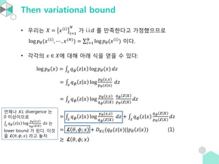
• (Eq.3) 𝓛 𝜃, 𝜙; 𝑥 = −𝐷 𝐾𝐿(𝑞 𝜙(𝑧|𝑥)||𝑝 𝜃 𝑥 ) + 𝐸 𝑞 𝜙 𝑧 𝑥 [log 𝑝 𝜃(𝑥|𝑧)]
<Proof>
𝓛 𝜃, 𝜙; 𝑥 = 𝑧
𝑞 𝜙 𝑧 𝑥 log
𝑝 𝜃(𝑧,𝑥)
𝑞 𝜙(𝑧|𝑥)
𝑑𝑧
= 𝑧
𝑞 𝜙 𝑧 𝑥 log
𝑝 𝜃 𝑧)𝑝 𝜃(𝑥|𝑧
𝑞 𝜙 (𝑧|𝑥)
𝑑𝑧
= 𝑧
𝑞 𝜙 𝑧 𝑥 log
𝑝 𝜃(𝑧)
𝑞 𝜙 (𝑧|𝑥)
𝑑𝑧 + 𝑧
𝑞 𝜙 𝑧 𝑥 log 𝑝 𝜃 𝑥 𝑧 𝑑𝑧
= −𝐷 𝐾𝐿(𝑞 𝜙(𝑧|𝑥)| 𝑝 𝜃(𝑧) + 𝐸 𝑞 𝜙 𝑧 𝑥 [log 𝑝 𝜃(𝑥|𝑧)]
𝑞 𝜙와 𝑝 𝜃가 normal 이면 계산 가능!
Reconstruction error](https://image.slidesharecdn.com/auto-encoders-180909040543/85/Auto-Encoders-and-Variational-Auto-Encoders-20-320.jpg)
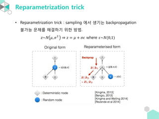
![Cost function
• Lemma. If 𝑝 𝑥 ~𝑁 𝜇1, 𝜎1
2
and 𝑞 𝑥 ~𝑁 𝜇2, 𝜎2
2
, then
𝐾𝐿(𝑝(𝑥)||𝑞 𝑥 ) = ln
𝜎2
𝜎1
+
𝜎1
2
+ 𝜇1 − 𝜇2
2
2𝜎2
2 −
1
2
• Corollary. 𝑞 𝜙 𝑧 𝑥 ~ 𝑁(𝜇𝑖, 𝜎𝑖
2
𝐼) 이고 𝑝 𝑧 ~𝑁 0,1 이면
𝐾𝐿 𝑞 𝜙 𝑧 𝑥𝑖 𝑝 𝑧 =
1
2
(𝑡𝑟 𝜎𝑖
2
𝐼 + 𝜇𝑖 𝑖
𝑇𝜇 − 𝐽 + ln
1
𝑗=𝑖
𝐽
𝜎𝑖,𝑗
2
)
= (Σ𝑗=1
𝐽
𝜎𝑖,𝑗
2
+ Σ𝑗=1
𝐽
𝜇𝑖,𝑗
2
− 𝐽 − Σ𝑗=1
𝐽
ln(𝜎𝑖,𝑗
2
))
=
1
2
Σ𝑗=1
𝐽
(𝜇𝑖,𝑗
2
+ 𝜎𝑖,𝑗
2
− 1 − ln 𝜎𝑖,𝑗
2
)
• 즉, 𝑞 𝜙 𝑧 𝑥 ~ 𝑁(𝜇𝑖, 𝜎𝑖
2
𝐼) 이고 𝑝 𝑧 ~𝑁 0,1 이면 Eq.3 는 아래와 같다.
𝓛 𝜃, 𝜙; 𝑥 =
1
2
Σ𝑗=1
𝐽
𝜇𝑖,𝑗
2
+ 𝜎𝑖,𝑗
2
− 1 − ln 𝜎𝑖,𝑗
2
+ 𝐸 𝑞 𝜙 𝑧 𝑥 [log 𝑝 𝜃(𝑥|𝑧)]](https://image.slidesharecdn.com/auto-encoders-180909040543/85/Auto-Encoders-and-Variational-Auto-Encoders-21-320.jpg)
![Reconstruction error 학습 방법
• 𝐸 𝑞 𝜙 𝑧 𝑥 [log 𝑝 𝜃(𝑥|𝑧)]는 sampling 을 통해 Monte-carlo estimation 한다.
즉, 𝑥𝑖 ∈ X 마다 𝑧 𝑖,1
, ⋯ , 𝑧 𝑖 𝐿 를 sampling 하여 log likelihood 의 mean으로
근사시킨다. 보통 𝐿 = 1 을 많이 사용한다.
𝐸 𝑞 𝜙 𝑧 𝑥 [log 𝑝 𝜃(𝑥|𝑧)] ∼
1
𝐿
Σ𝑙=1
𝐿
log(𝑝 𝜃 𝑥𝑖 𝑧 𝑖,𝑙 )
• 이렇게 sampling 을 하면 backpropagation 을 할 수 없다. 그래서 사용
되는 방법이 reparametrization trick 이다.
𝑞 𝜙 𝑥 𝑧 𝑝 𝜃 𝑥 𝑧](https://image.slidesharecdn.com/auto-encoders-180909040543/85/Auto-Encoders-and-Variational-Auto-Encoders-22-320.jpg)
![Log Likelihood
• 앞에서 reconstruction error 를 계산할 때 하나씩 sampling 을 하면
𝐸 𝑞 𝜙 𝑧 𝑥 [log 𝑝 𝜃(𝑥|𝑧)] ∼
1
𝐿
Σ𝑙=1
𝐿
log 𝑝 𝜃 𝑥𝑖 𝑧 𝑖,𝑙
= log(𝑝 𝜃(𝑥𝑖|𝑧 𝑖
)
가 된다. 여기서 𝑝 𝜃 𝑥𝑖 𝑧 𝑖
의 분포가 Bernoulli 인 경우에 아래의 식을
얻을 수 있다.
출처 : https://github.com/hwalsuklee/tensorflow-mnist-VAE](https://image.slidesharecdn.com/auto-encoders-180909040543/85/Auto-Encoders-and-Variational-Auto-Encoders-24-320.jpg)
![References
• [VLBM] Extracting and composing robust features with denoising
autoencoders, Vincent, Larochelle, Bengio, Manzagol, 2008
• [KW] Auto-Encoding Variational Bayes, Diederik P Kingma, Max
Welling, 2013
• [D] Tutorial on Variational Autoencoders - Carl Doersch, 2016
• PR-010: Auto-Encoding Variational Bayes, ICLR 2014, 차준범
• 오토인코더의 모든 것, 이활석
https://github.com/hwalsuklee/tensorflow-mnist-VAE](https://image.slidesharecdn.com/auto-encoders-180909040543/85/Auto-Encoders-and-Variational-Auto-Encoders-30-320.jpg)


![[신경망기초] 소프트맥스회귀분석](https://cdn.slidesharecdn.com/ss_thumbnails/nn09-180318142813-thumbnail.jpg?width=640&height=640&fit=bounds)


![[신경망기초] 멀티레이어퍼셉트론](https://cdn.slidesharecdn.com/ss_thumbnails/nn04-180318141650-thumbnail.jpg?width=640&height=640&fit=bounds)
![[신경망기초] 오류역전파알고리즘](https://cdn.slidesharecdn.com/ss_thumbnails/nn06-180318141901-thumbnail.jpg?width=640&height=640&fit=bounds)


![[신경망기초] 선형회귀분석](https://cdn.slidesharecdn.com/ss_thumbnails/nn07-180318142107-thumbnail.jpg?width=640&height=640&fit=bounds)


![[한글] Tutorial: Sparse variational dropout](https://cdn.slidesharecdn.com/ss_thumbnails/tutorialsparsevariationaldropout-190728122300-thumbnail.jpg?width=640&height=640&fit=bounds)