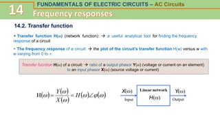
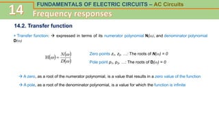
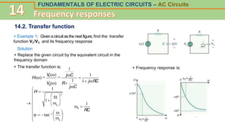
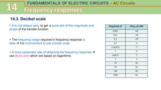
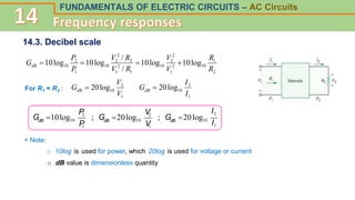
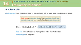
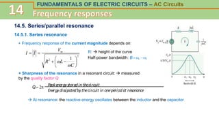
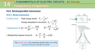
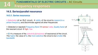
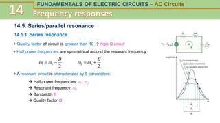
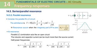
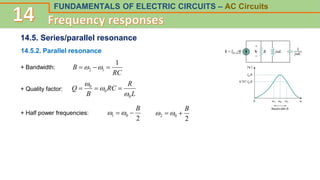
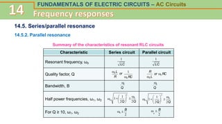
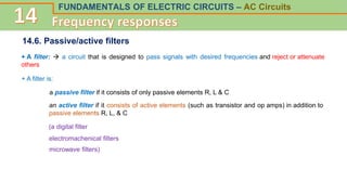
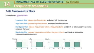
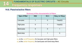
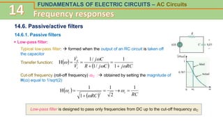
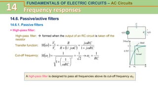
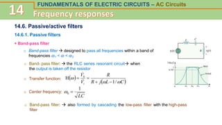
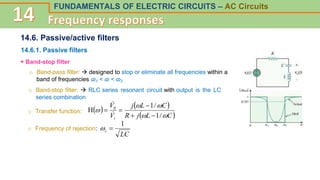
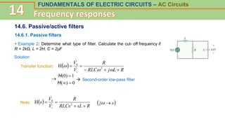
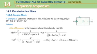
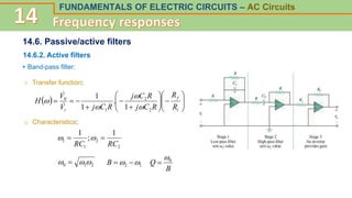
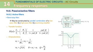
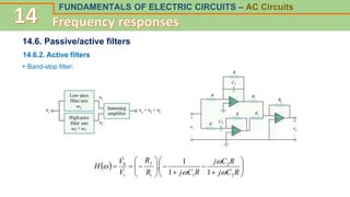
LC2-EE3726-C14-Frequency_responses.pdf

Fundamentals of Electric Circuits
AC Circuits
Chapter 14. Frequency responses
14.1. Introduction
14.2. Transfer function
14.3. Decibel scale
14.4. Bode plots
14.5. Series/parallel resonance
14.6. Passive/active filters
14.7. Scaling

FUNDAMENTALS OF ELECTRIC CIRCUITS – AC Circuits
14.1. Introduction
+ Previous chapters: learned how to find voltages and currents in a circuit with a constant frequency
source
+ Let the amplitude of the sinusoidal source remain constant and vary the frequency  obtain the
circuit’s frequency response
The frequency response of a circuit is the variation in its
behavior with change in signal frequency
+ The sinusoidal steady state frequency responses of circuits  significant in many applications
(communications, control systems, filters)

+ Transfer function H(ɷ) (network function):  a useful analytical tool for finding the frequency
response of a circuit
+ The frequency response of a circuit:  the plot of the circuit’s transfer function H(w) versus w with
w varying from 0 to ∞
Transfer fucntion H(ɷ) of a circuit:  ratio of a output phasor Y(ɷ) (voltage or current on an element)
to an input phasor X(ɷ) (source voltage or current)
Linear network
.
H()
.
X()
Input
.
Y()
Output
   
 
   





 

 H
X
Y
H

+ Since the input and output can be either voltage or current  4 possible transfer functions
Voltage gain:    
 



i
o
V
V



H Current gain:    
 



i
o
I
I



H
Transfer impedance:    
 



i
o
I
V



H Transfer admittance:    
 



i
o
V
I



H
+ To obtain the transfer functions:
o Replace: R
R  L
j
L 

C
j
C

1

o Apply any circuit analysis technique to find the defined ratio

+ Transfer function:  expressed in terms of its numerator polynomial N(ɷ), and denominator polynomial
D(ɷ)
Zero points z1, z2, …: The roots of N(ɷ) = 0
Pole point p1, p2, …: The roots of D(ɷ) = 0
   
 



D
N

H
 A zero, as a root of the numerator polynomial, is a value that results in a zero value of the function
 A pole, as a root of the denominator polynomial, is a value for which the function is infinite

+ Example 1: Given a circuit as the next figure, find the transfer
function V0/VS and its frequency response
+ Replace the given circuit by the equivalent circuit in the
frequency domain
Solution
+ The transfer function is:

V
0 ()
 jC
H()
1 jRC
V ()
jC

R
S
.
.
.
1
1
1
  
1  
  tan1   
 
H 


 
  0 

  0 

2
1
 
RC
0
1
+ Frequency response is:

14.3. Decibel scale
Magnitude H 20log10H (dB)
0,001 -60
0,01 -40
0,1 -20
0,5 -6
1/sqrt(2) -3
1 0
sqrt(2) 3
2 6
10 20
20 26
100 40
1000 60
+ It is not always easy to get a quick plot of the magnitude and
phase of the transfer function
+ A more systematic way of obtaining the frequency response 
use Bode plots which are based on logarithms
+ The frequency range required in frequency response is
wide  it is inconvenient to use a linear scale

14.3. Decibel scale
2
1
10
2
1
2
2
10
1
2
1
2
2
2
10
1
2
10 log
10
log
10
/
/
log
10
log
10
R
R
V
V
R
V
R
V
P
P
GdB 



1
2
10
log
20
V
V
GdB 
For R1 = R2 :
1
2
10
log
20
I
I
GdB 
G 10log10 ; G 20log10 ; G 20log10
dB dB dB
P
2 V
2
I2
I1
P
1 V
1
+ Note:
o 10log is used for power, which 20log is used for voltage or current
o dB value is dimensionless quantity

14.4. Bode plot
+ In Bode plots:  a logarithmic scale for the frequency axis, a linear scale in magnitude or phase
Bode plots are semilog plots of the magnitude (in dB) and
phase (in degrees) of a transfer function versus frequency
       
      




 

j
H
e
H
He
H j
j







 ln
ln
ln
H
ln
H
Real part lnH is a function of the magnitude of the transfer function
Imaginary part is the phase

+ The most prominent feature of the frequency response:  the sharp peak (resonant peak) exhibited in its
amplitude characteristic
+ Resonance occurs:
 in any system that has a complex conjugate pair of poles
 cause of oscillations of stored energy from one form to another
+ Resonance is a phenomenon:  allows frequency discrimination in communication networks, filter
construction,…
Resonance is a condition in an R-L-C circuit in which the capacitive and inductive impedance are
equal in magnitude, thereby resulting in a purely resistive impedance (reactance equals to zero)

14.5.1. Series resonance
+ Consider the series RLC circuit:
Input impedance   










C
L
j
R
I
V
Z s



1
H


When resonance
 
LC
f
LC
C
L
Z




2
1
1
0
1
Im 0
0 





 ɷ0: resonant frequency
At resonance:
o The impedance is purely resistive, L-C series combination acts like a short circuit, and the
entire voltage is across R
o Voltage VS, current I are in phase, the power factor is unity
o H(ɷ) = Z(ɷ) is minimum
o VL, and VC can be much more than the source voltage

+ The frequency response of the current magnitude:
2
2 1










C
L
R
V
I
I m



+ The highest power dissipated:  
R
V
P m
2
0
2
1


+ The half-power frequencies:    
R
V
P
P m
4
2
2
1 
 

LC
L
R
L
R 1
2
2
2
1 










LC
L
R
L
R 1
2
2
2
2 









+ Relationship between resonant frequency & half-power frequencies: 2
1
0 

 

+ Frequency response of the current magnitude depends on:
2
2 1










C
L
R
V
I
I m


 R:  height of the curve
Half-power bandwidth: B 2 1
+ Sharpness of the resonance in a resonant circuit:  measured
by the quality factor Q
Q  2
Peakenergystoredinthecircuit
Energydissipatedbythecircuit in oneperiodat resonance
 At resonance: the reactive energy oscillates between the inductor and the capacitor

+ In RLC circuit: Peak energy stored:
Energy dissipated in one period:
2
2
1
LI
Ep 
f
RI
Ed
2
2
1

+ Quality factor Q:
R
fL
f
RI
LI
Q


2
2 2
2


RC
R
L
Q
0
0 1




+ Relationship between B and Q: RC
Q
L
R
B 2
0
0





The quality factor of a resonant circuit is the ratio of its
resonant frequency to its bandwidth

+ Selectivity (of an RLC circuit):  ability of the circuit to respond to a
certain frequency and discriminate against all other frequencies
+ (Selected or rejected) Frequency Band  narrow / wide, Quality factor of
the resonant circuit  high / low
+ Q  a measure of the selectivity (sharpness of resonance) of the circuit.
The higher the value of Q, the more selective the circuit is but smaller the
bandwidth

+ Quality factor of circuit is greater than 10  high-Q circuit
+ Half power frequencies are symmetrical around the resonant frequency
2
0
1
B

 

2
0
2
B

 

+ A resonant circuit is characterized by 5 parameters:
 Half-power frequencies: ɷ1, ɷ2
 Resonant frequency: ɷ0
 Bandwidth B
 Quality factor Q

14.5.2. Parallel resonance
+ Consider the parallel R-L-C circuit:
The admittance is:  
L
j
C
j
R
V
I
Y



1
1
H 






 Resonance occurs when the imaginary part of Y is zero
+ At resonance:
Parallel LC combination acts like an open circuit
The inductor and capacitor current can be much more than the source current
Half-power frequencies:
LC
RC
RC
1
2
1
2
1
2
1 










LC
RC
RC
1
2
1
2
1
2
2 









LC
1
0 


+ Bandwidth:
RC
B
1
1
2 

 

+ Quality factor:
L
R
RC
B
Q
0
0
0






+ Half power frequencies:
2
0
1
B

 

2
0
2
B

 


Summary of the characteristics of resonant RLC circuits
Characteristic Series circuit Parallel circuit
Bandwidth, B
Half power frequencies, ω1, ω2
For Q ≥ 10, ω1, ω2
0
Q
0
Q
1
 1 

0
2Q
  
 2Q
2
0
Resonant frequency, ω0
Quality factor, Q
1 1
LC LC
0 L
or
 RC  L
R 0
1 R
or 0 RC
0

 1  0
0 1  

 2Q 2Q
2
0 
2
B  
0
2
B

+ A filter:  a circuit that is designed to pass signals with desired frequencies and reject or attenuate
others
+ A filter is:
a passive filter if it consists of only passive elements R, L & C
an active filter if it consists of active elements (such as transistor and op amps) in addition to
passive elements R, L, & C
(a digital filter
electromachenical filters
microwave filters)

+ There are 4 types of filters:
Low-pass filter: passes low frequencies and stop high frequencies
High-pass filter: passes high frequencies and reject low frequencies
Band-pass filter: passes frequencies within a frequency band and block or attenuates frequencies
outsides the band
Band-stop filter: passes frequencies outside a frequency band and block or attenuates
frequencies within the band

Summary of the characteristics of filters
Type of filter H(0) H(∞) H(ɷC) or H(ɷ0)
Low-pass 1 0 1/sqrt(2)
High-pass 0 1 1/sqrt(2)
Band-pass 0 0 1
Band-stop 1 1 0
ɷC is the cut-off frequency for low-pass and high-pass filters
ɷ0 is the center frequency for band-pass and band-stop filters

14.6.1. Passive filters
+ Low-pass filter:
Typical low-pass filter:  formed when the output of an RC circuit is taken off
the
. capacitor
Transfer function:  
  RC
j
C
j
R
C
j
V
V
i 








1
1
/
1
/
1
H 0


Cut-off frequency (roll-off frequency) ɷC : obtained by setting the magnitude of
H(ɷ) equal to 1/sqrt(2)
 
  RC
RC
c
c
1
2
1
1
1
H
2




 


Low-pass filter is designed to pass only frequencies from DC up to the cut-off frequency ɷC

+ High-pass filter:
High-pass filter:  formed when the output of an RC circuit is taken off the
resistor
  RC
j
RC
j
C
j
R
R
V
V
i 








1
/
1
H 0


Cut-off frequency:  
RC
RC
c
c
1
2
1
1
1
1
H
2










 


A high-pass filter is designed to pass all frequencies above its cut-off frequency ɷC

+ Band-pass filter
o Band- pass filter:  the RLC series resonant circuit when
the output is taken off the resistor
o Transfer function:  
 
C
L
j
R
R
V
V
i 


/
1
H 0






o Center frequency:
LC
1
0 

o Band-pass filter  designed to pass all frequencies within a band of
frequencies ɷ1 < ɷ < ɷ2
o Band-pass filter:  also formed by cascading the low-pass filter with the high-pass
filter

+ Band-stop filter
o Band-pass filter:  designed to stop or eliminate all frequencies within a
band of frequencies ɷ1 < ɷ < ɷ2
o Band-stop filter:  RLC series resonant circuit with output is the LC
series combination
o Transfer function:    
 
C
L
j
R
C
L
j
V
V
i 




/
1
/
1
H 0







o Frequency of rejection:
LC
c
1



+ Example 2: Determine what type of filter. Calculate the cut- off frequency if
R = 2kΩ, L = 2H, C = 2µF
Solution
R
L
j
RLC
R
V
V
i 






 2
0
H



H(0) 1
H()  0
 Second-order low-pass filter
Note:  
R
sL
RLCs
R
V
V
s
i 


 2
0
H


 
s
j 


+ Example 2: Determine what type of filter. Calculate the cut- off frequency if
R = 2kΩ, L = 2H, C = 2µF
Solution
+ Cut-off frequency is the frequency where H is reduce by 1/sqrt(2):
 
  2
2
2
2
2
0
H
L
RLC
R
R
H
R
L
j
RLC
R
V
V
i 















  2
2
2
2
2
2
2
1
L
RLC
R
R
H
c
c 
 



 s
rad
c
c
c /
742
0
1
7
16 2
2





 



+ Three major limits of the passive filters:
o Cannot generate gain greater than 1 Passive elements cannot add energy to the
network
o May require bulky and expensive inductor
o Perform poorly at frequencies below the audio frequency range (300Hz < f < 3000Hz) (the
passive filters are useful at high frequencies)

14.6.2. Active filters
+ Active filters consist of combinations of R, C & Op-Amps  offer some advantages over passive RLC
filters
 Often smaller and less expensive because they do not require inductor
 Can provide amplifier gain in addition to providing the same frequency response as RLC filters
 Can be combined with buffer amplifier (voltage followers) to isolate each stage of the filter from
source and load impedance effects
+ Active filters are less reliable, less stable, & limit at low frequency (<100kHz)

+ One type of first-order active filter:
Components Zi and Zf
 One of them must be reactive
 They determine whether the filter is low-pass or high-pass
+ First-order low-pass filter:
f
f
i
f
i
f
i R
C
j
R
R
Z
Z
V
V
H








1
1
.
0


Cut-off frequency:
f
f
c
C
R
1



+ First-order high-pass filter:
o Transfer function:  
i
i
f
i
i
f
i R
C
j
R
C
j
Z
Z
V
V
H









1
0


o Cut-off frequency:
i
i
c
C
R
1


+ Band-pass filter:
To form a band-pass filter: combine an unity-gain low-pass filter with
unity-gain high-pass filter & an inverter with gain - Rf/Ri

+ Band-pass filter:
o Transfer function:
  






















i
f
i R
R
R
C
j
R
C
j
R
C
j
V
V
H
2
2
1
0
1
.
1
1



 

o Characteristics:
2
2
1
1
1
;
1
RC
RC

 

2
1
0 

  1
2 
 

B
B
Q 0



+ Band-stop filter:
 May be constructed by parallel combination of a low-
pass filter & a high-pass filter & a summing amplifier
o Transfer function:
  






















R
C
j
R
C
j
R
C
j
R
R
V
V
H
i
f
i 2
2
1
0
1
1
1
.



 

o Characteristics:
2
2
1
1
1
;
1
RC
RC

 

2
1
0 

  1
2 
 

B
B
Q 0



+ Band-stop filter:
  






















R
C
j
R
C
j
R
C
j
R
R
V
V
H
i
f
i 2
2
1
0
1
1
1
.



 


14.7. Scaling
+ In designing or analyzing filters and resonant circuits (circuit analysis in general): it is sometimes
convenient to work with:
Element values of 1Ω, 1H, 1F
Then transform to realistic values by scaling
+ Two ways of scaling a circuit:
o Magnitude or impedance scaling:  increasing all impedance in a network by a factor; the
frequency response remaining unchanged
o Frequency scaling:  shifting the frequency response of a network up or down the frequency axis
while leaving the impedance the same

LC2-EE3726-C14-Frequency_responses.pdf

More Related Content

What's hot

Similar to LC2-EE3726-C14-Frequency_responses.pdf

Recently uploaded

LC2-EE3726-C14-Frequency_responses.pdf