Download to read offline


![Two Security Case (cont’d)
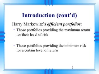
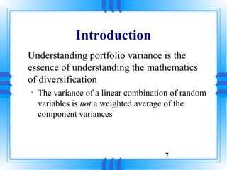
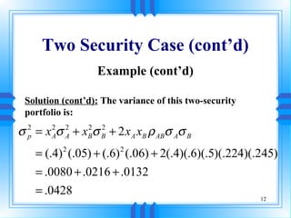
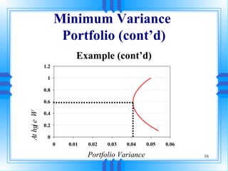
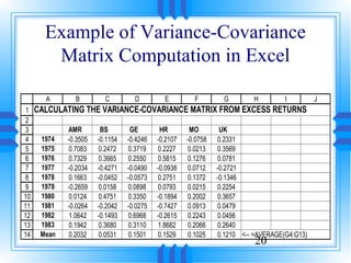
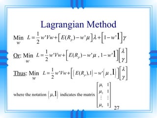
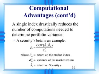
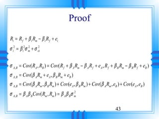
Example (cont’d)
Solution: The expected return of this two-security
portfolio is: n
E ( R p ) = ∑ xi E ( Ri )
%
%
i =1
= x A E ( RA ) + xB E ( RB )
%
%
= [ 0.4(0.015) ] + [ 0.6(0.020) ]
= 0.018 = 1.80%
11](https://image.slidesharecdn.com/ch05-130306041313-phpapp02/85/Ch05-11-320.jpg)
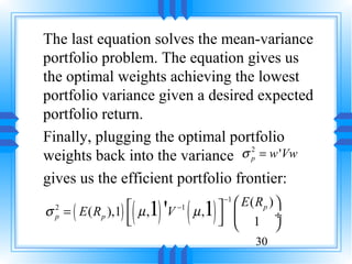
![A B C D E F G H I J K
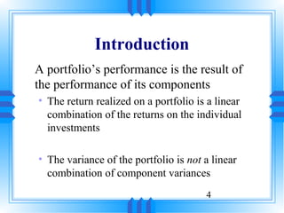
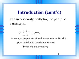
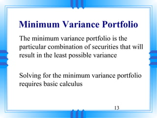
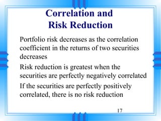
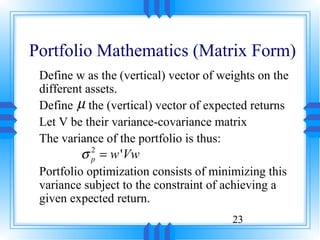
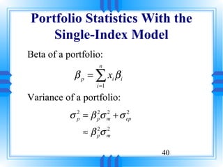
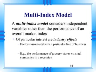
16 Excess return matrix
17 AMR BS GE HR MO UK
18 1974 -0.5537 -0.1686 -0.5747 -0.3635 -0.1784 0.1121
19 1975 0.5051 0.1940 0.2218 0.0698 -0.0812 0.2359
20 1976 0.5297 0.3134 0.1049 0.4286 0.0250 -0.0429
21 1977 -0.4066 -0.4802 -0.1991 -0.2466 -0.0313 -0.3931
22 1978 -0.0369 -0.0984 -0.2074 0.1222 0.0347 -0.2555
23 1979 -0.4691 -0.0374 -0.0603 -0.0736 -0.0810 0.1044
24 1980 -0.1908 0.4220 0.1849 -0.3423 0.0977 0.2447
25 1981 -0.2296 -0.2574 -0.1777 -0.8956 -0.0112 -0.0731
26 1982 0.8610 -0.2024 0.5467 -0.4144 0.1217 -0.0754 <-- =G12-$G$14
27 1983 -0.0090 0.3149 0.1609 1.7154 0.1041 0.1430 <-- =G13-$G$14
28
29 Transpose of excess return matrix
30 1974 1975 1976 1977 1978 1979 1980 1981 1982 1983
31 AMR -0.5537 0.5051 0.5297 -0.4066 -0.0369 -0.4691 -0.1908 -0.2296 0.8610 -0.0090
32 BS -0.1686 0.1940 0.3134 -0.4802 -0.0984 -0.0374 0.4220 -0.2574 -0.2024 0.3149
33 GE -0.5747 0.2218 0.1049 -0.1991 -0.2074 -0.0603 0.1849 -0.1777 0.5467 0.1609
34 HR -0.3635 0.0698 0.4286 -0.2466 0.1222 -0.0736 -0.3423 -0.8956 -0.4144 1.7154
35 MO -0.1784 -0.0812 0.0250 -0.0313 0.0347 -0.0810 0.0977 -0.0112 0.1217 0.1041
36 UK 0.1121 0.2359 -0.0429 -0.3931 -0.2555 0.1044 0.2447 -0.0731 -0.0754 0.1430
37 Cells B31:K36 contain the array formula =TRANSPOSE(B18:G27). To
38 enter this formula:
39 1. Mark the area B31:K36
40 2. Type =TRANSPOSE(B18:G27)
41 3. Instead of [Enter], finish with [Ctrl]-[Shift]-[Enter]
42 The formula will appear as {=TRANSPOSE(B18:G27)}
43
21](https://image.slidesharecdn.com/ch05-130306041313-phpapp02/85/Ch05-21-320.jpg)
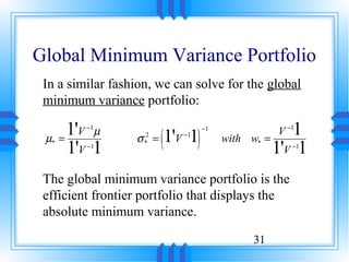
![A B C D E F G H
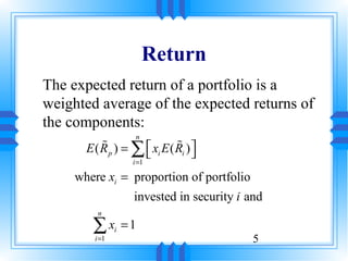
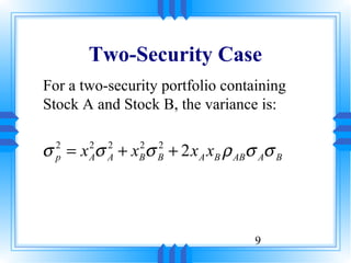
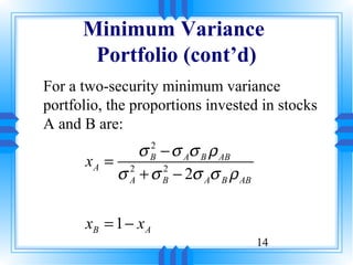
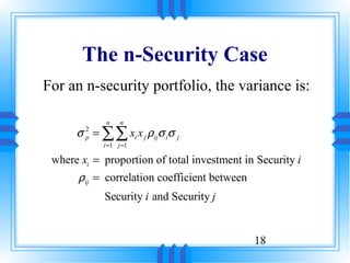
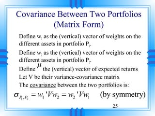
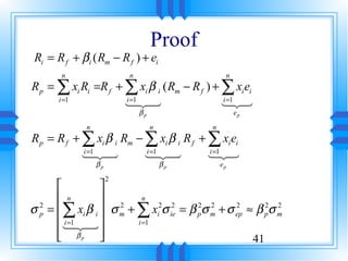
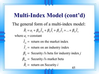
45 Product of transpose[excess return] times [excess return] / 10
46 AMR BS GE HR MO UK
47 AMR 0.2060 0.0375 0.1077 0.0493 0.0208 0.0059
48 BS 0.0375 0.0790 0.0355 0.1028 0.0089 0.0406
49 GE 0.1077 0.0355 0.0867 0.0443 0.0194 0.0148
50 HR 0.0493 0.1028 0.0443 0.4435 0.0193 0.0274
51 MO 0.0208 0.0089 0.0194 0.0193 0.0083 -0.0015
52 UK 0.0059 0.0406 0.0148 0.0274 -0.0015 0.0392
53
Cells B47:G52 contain the array formula =MMULT(B31:K36,B18:G27)/10 . To
54
enter this formula:
55
1. Mark the whole area
56
2. Type =MMULT(B31:K36,B18:G27)/10
57
3. Instead of [Enter], finish with [Ctrl]-[Shift]-[Enter]
58
The formula will appear as {=MMULT(B31:K36,B18:G27)/10}
59
22](https://image.slidesharecdn.com/ch05-130306041313-phpapp02/85/Ch05-22-320.jpg)
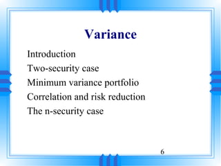
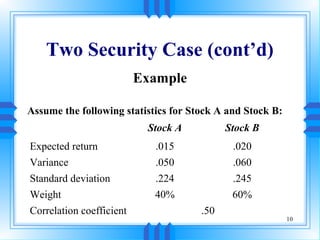
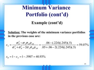
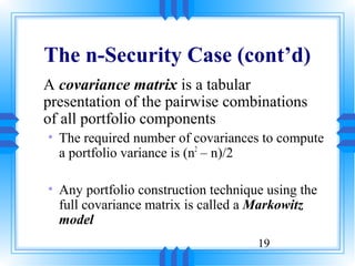
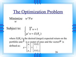
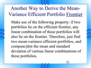
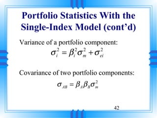
![Portfolio Variance in the 2-asset case
We have:
wA σ A σ AB
2
w= and V = 2
wB σ AB σ B
Hence:
σ A σ AB wA
2
σ p = w 'Vw = [ wA wB ]
2
2
σ AB σ B wB
σ p = wAσ A + wBσ B + 2wA wBσ AB
2 2 2 2 2
σ p = wAσ A + wBσ B + 2wA wB ρ ABσ Aσ B
2 2 2 2 2
24](https://image.slidesharecdn.com/ch05-130306041313-phpapp02/85/Ch05-24-320.jpg)
![Taking Derivatives
∂L
∂w
( 1) λ
= Vw − µ , = 0 ⇒ w = V µ ,
γ
−1 λ
γ
( 1) (1)
∂L
0 ∂L ( 1)
0 = ∂λ ⇒ E ( R ),1 − w ' µ , = 0, 0
( p ) ( ) (2)
∂γ
Plugging (1) into (2) yields:
µ ' −1
1'
( 1) = ( 0, 0)
( E ( Rp ),1) − [ λ , γ ] V µ ,
28](https://image.slidesharecdn.com/ch05-130306041313-phpapp02/85/Ch05-28-320.jpg)
![And so we have:
−1
µ ' −1
1'
( 1)
[ λ , γ ] = ( E ( Rp ),1) V µ ,
In other words:
λ
( 1) ' ( 1) E ( Rp )
−1
γ = µ , V µ , 1
−1
Plugging the last expression back into (1) finally yields:
−1
{ { ( 1) ( 1) '
−1
w = V × µ , × µ , ×{ × µ , ×
V −1
( 1) E (Rp )
1 3 ( n×n ) { 4 3 1
( n×1) ( n× n ) { 2 1 24
1 24 (2×n ) 2444
4 ( n×3 1444
2) ( n×2)
3 (2×1)
( n×2)
14444444 (2×2) 4 244444444 3
( n×1) 29](https://image.slidesharecdn.com/ch05-130306041313-phpapp02/85/Ch05-29-320.jpg)
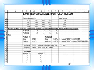
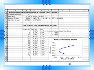


The document discusses portfolio theory and diversification from a mathematical perspective. It introduces portfolio variance and how diversifying investments reduces risk. The variance of a portfolio is not a linear combination of the component variances due to correlation between investments. Harry Markowitz's efficient portfolios provide the maximum return for a given level of risk or minimum risk for a given level of return through diversification.