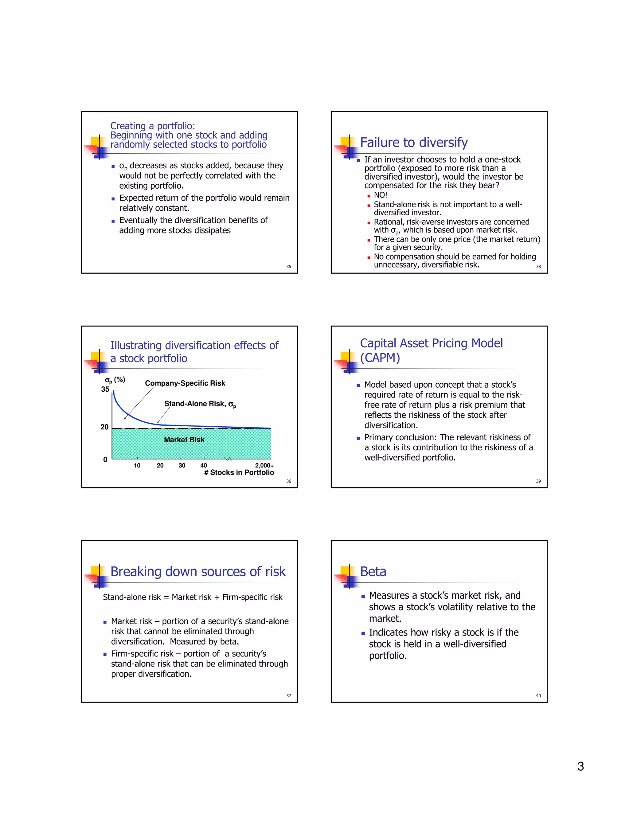
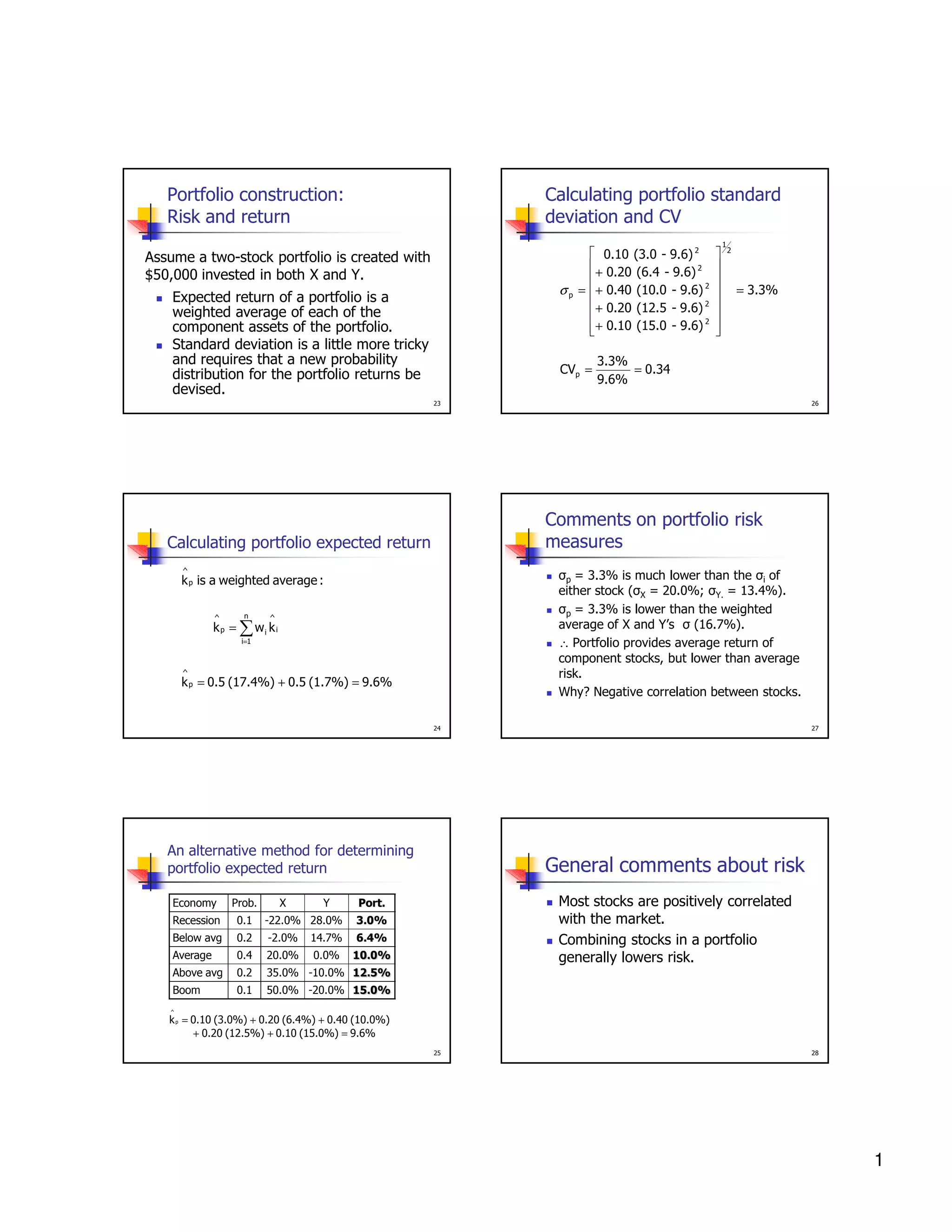
- Portfolio risk is calculated using the weighted average of the component assets' standard deviations and their correlations. Diversification reduces overall portfolio risk even when holding riskier individual assets. - The expected return of a portfolio is the weighted average of the individual assets' expected returns. Standard deviation requires determining a new probability distribution for portfolio returns. 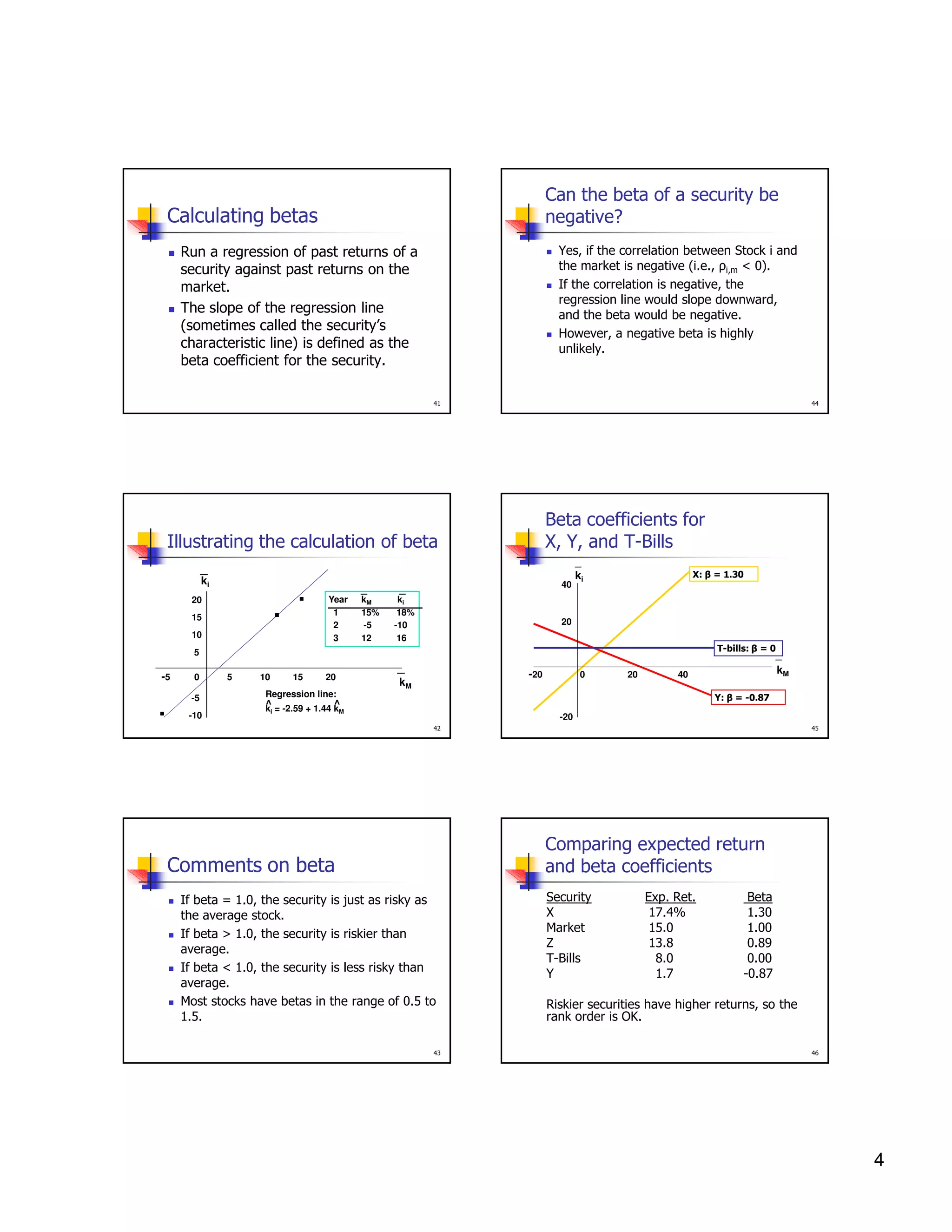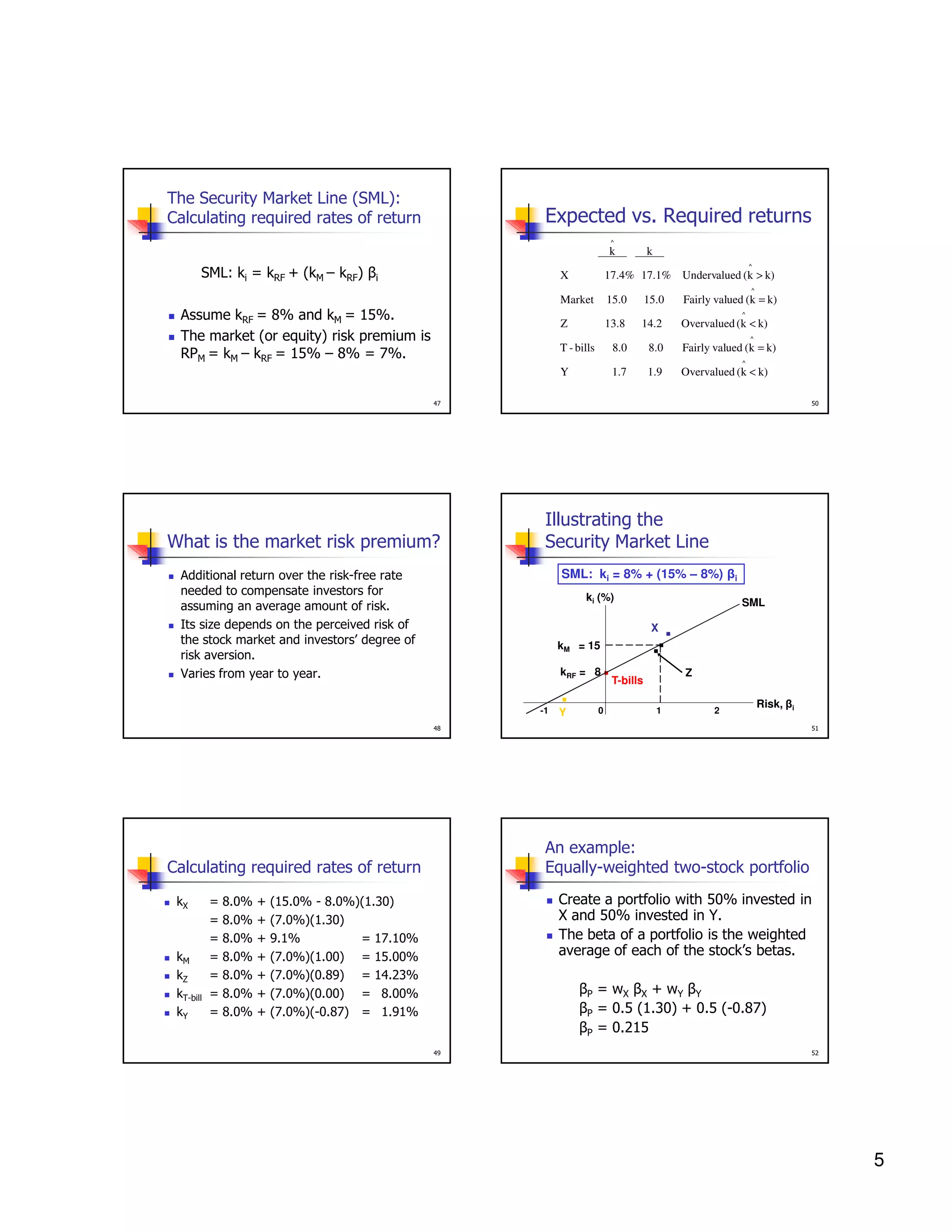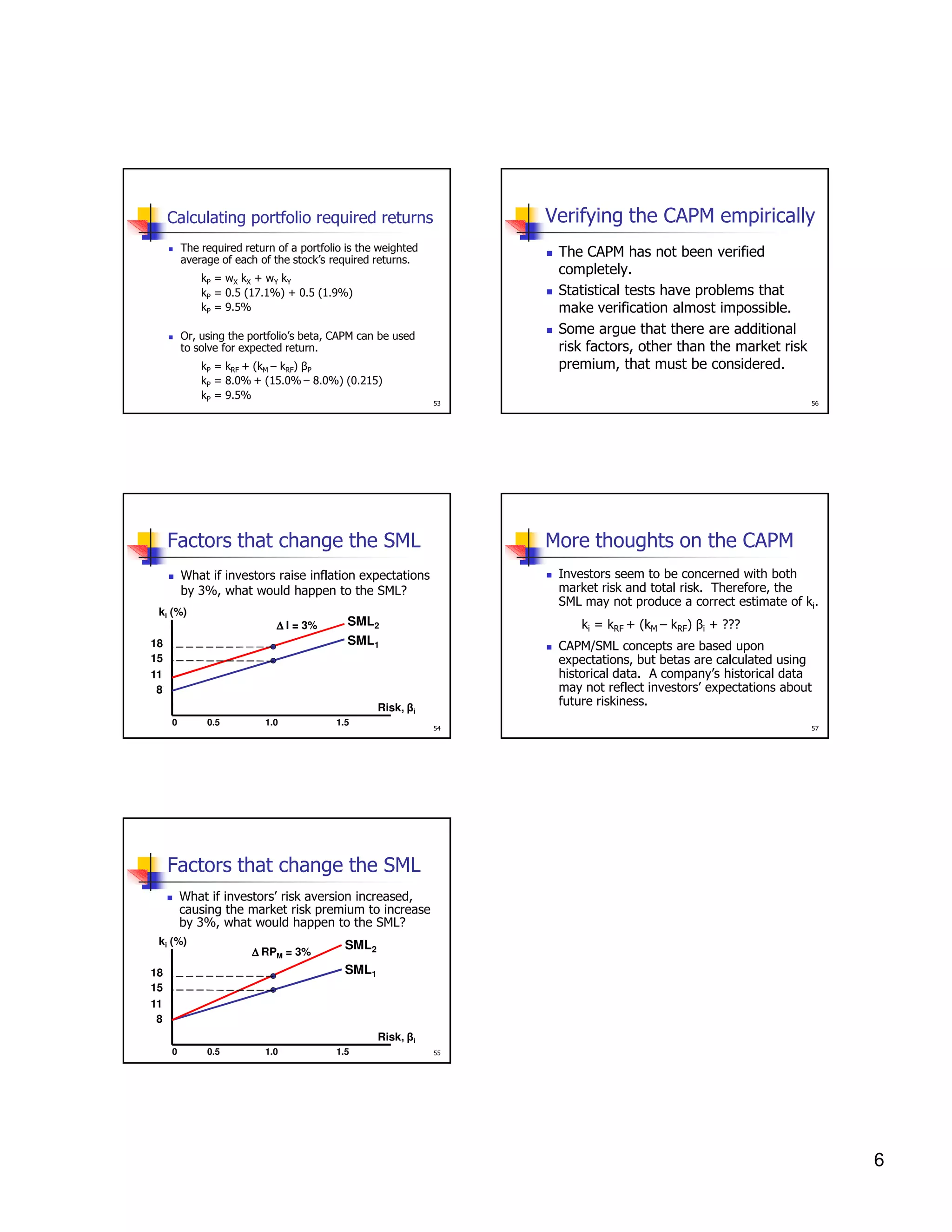- The Capital Asset Pricing Model (CAPM) states that the expected return of an asset is determined by its beta coefficient, which measures non-diversifiable market risk relative to the overall market. The Security Market Line plots the relationship between risk and return based on the CAPM.

1. Portfolio construction:
Risk and return
Calculating portfolio standard
deviation and CV
 0.10 (3.0 - 9.6) 2
 + 0.20 (6.4 - 9.6) 2

σ p =  + 0.40 (10.0 - 9.6) 2
 + 0.20 (12.5 - 9.6) 2

2
 + 0.10 (15.0 - 9.6)

Assume a two-stock portfolio is created with
$50,000 invested in both X and Y.
Expected return of a portfolio is a
weighted average of each of the
component assets of the portfolio.
Standard deviation is a little more tricky
and requires that a new probability
distribution for the portfolio returns be
devised.
CVp =








1
2
= 3.3%
3.3%
= 0.34
9.6%
23
Comments on portfolio risk
measures
Calculating portfolio expected return
^
σp = 3.3% is much lower than the σi of
either stock (σX = 20.0%; σY. = 13.4%).
σp = 3.3% is lower than the weighted
average of X and Y’s σ (16.7%).
∴ Portfolio provides average return of
component stocks, but lower than average
risk.
Why? Negative correlation between stocks.
k p is a weighted average :
^
n
26
^
k p = ∑ wi k i
i=1
^
k p = 0.5 (17.4%) + 0.5 (1.7%) = 9.6%
24
An alternative method for determining
portfolio expected return
Economy
Prob.
Recession
0.1
X
Y
-22.0% 28.0%
General comments about risk
Most stocks are positively correlated
with the market.
Combining stocks in a portfolio
generally lowers risk.
Port.
3.0%
Below avg
0.2
-2.0%
14.7%
6.4%
Average
0.4
20.0%
0.0%
10.0%
Above avg
0.2
35.0% -10.0% 12.5%
Boom
0.1
27
50.0% -20.0% 15.0%
^
k p = 0.10 (3.0%) + 0.20 (6.4%) + 0.40 (10.0%)
+ 0.20 (12.5%) + 0.10 (15.0%) = 9.6%
25
28
1

2. Returns distribution for two perfectly
negatively correlated stocks (ρ = -1.0)
Covx,y & Corr x,y ?
A
Stock W
Stock M
Economy
25
25
25
15
15
15
0
0
0
-10
-10
Prob.
RX
0.1
0.2
0.4
0.2
0.1
-22%
-2%
20%
35%
50%
28%
15%
0%
-10%
-20%
17.4%
20.00%
C
1.7%
13.40%
Ex. Return
Std.dev
Covariance (x,Y)
-10
B
Ry
Recession
Below avg
Average
Above avg
Boom
Portfolio WM
A*B
RX -E(Rx) RY-E(RY)
-39.4% 26.3%
-19.4% 13.0%
2.6% -1.7%
17.6% -11.7%
32.6% -21.7%
-10.36%
-2.52%
-0.04%
-2.06%
-7.07%
C* Prob
-1.04%
-0.50%
-0.02%
-0.41%
-0.71%
-2.68%
Corr (x,Y)
-1.00
29
Incorporating correlation to
portfolio risk calculation
Returns distribution for two perfectly
positively correlated stocks (ρ = 1.0)
Stock M’
Stock M
2
σ p = Wx 2 *σ 2 + W y2 * σ y + 2WxW y Corrxyσ xσ y
x
Portfolio MM’
25
25
15
15
0
0
0
-10
-10
OR, using covariance
25
15
32
-10
2
σ p = Wx 2 *σ 2 + W y2 *σ y + 2WxW y Cov xy
x
Previous Example,
σ p = 0.5 2 * 20 2 + 0.5 2 *13.4 2 + 2 * 0.5 * 0.5 * −1* 20 *13.4
2
30
Co var iance ( X , Y )
σ x *σ y
Cov ( x , y ) = Corr ( x , y ) * σ
x
*σ
33
Calculate the portfolio risk and return
for the example 2 given above if 60%
of investment is made on stock P
,
Therefore
σ p = 0.5 * 20 2 + 0.52 *13.4 2 + 2 * 0.5 * 0.5 * −2.68
σ p = 3. 3
Portfolio risk and return using
historical data
How to find correlation ?
Corr ( x , y ) =
OR, using covariance
σ p = 3. 3
y
Covariance for forecast data with probabilities
n
Cov ( x , y ) =
∑ [r
x
− E ( r x )] [ r y − E ( r y )] Pi
i =1
Covariance for historical data
∑ ( x − x)( y
i
Cov( x, y ) =
i
− y)
i =1
n −1
31
34
2

3. Creating a portfolio:
Beginning with one stock and adding
randomly selected stocks to portfolio
Failure to diversify
σp decreases as stocks added, because they
would not be perfectly correlated with the
existing portfolio.
Expected return of the portfolio would remain
relatively constant.
Eventually the diversification benefits of
adding more stocks dissipates
35
Company-Specific Risk
Model based upon concept that a stock’s
required rate of return is equal to the riskfree rate of return plus a risk premium that
reflects the riskiness of the stock after
diversification.
Primary conclusion: The relevant riskiness of
a stock is its contribution to the riskiness of a
well-diversified portfolio.
Stand-Alone Risk, σp
20
Market Risk
0
10
20
30
40
NO!
Stand-alone risk is not important to a welldiversified investor.
Rational, risk-averse investors are concerned
with σp, which is based upon market risk.
There can be only one price (the market return)
for a given security.
No compensation should be earned for holding
unnecessary, diversifiable risk.
38
Capital Asset Pricing Model
(CAPM)
Illustrating diversification effects of
a stock portfolio
σp (%)
35
If an investor chooses to hold a one-stock
portfolio (exposed to more risk than a
diversified investor), would the investor be
compensated for the risk they bear?
2,000+
# Stocks in Portfolio
36
Breaking down sources of risk
39
Beta
Stand-alone risk = Market risk + Firm-specific risk
Market risk – portion of a security’s stand-alone
risk that cannot be eliminated through
diversification. Measured by beta.
Firm-specific risk – portion of a security’s
stand-alone risk that can be eliminated through
proper diversification.
37
Measures a stock’s market risk, and
shows a stock’s volatility relative to the
market.
Indicates how risky a stock is if the
stock is held in a well-diversified
portfolio.
40
3

4. Can the beta of a security be
negative?
Calculating betas
Yes, if the correlation between Stock i and
the market is negative (i.e., ρi,m < 0).
If the correlation is negative, the
regression line would slope downward,
and the beta would be negative.
However, a negative beta is highly
unlikely.
Run a regression of past returns of a
security against past returns on the
market.
The slope of the regression line
(sometimes called the security’s
characteristic line) is defined as the
beta coefficient for the security.
41
44
Beta coefficients for
X, Y, and T-Bills
Illustrating the calculation of beta
_
ki
20
.
15
.
10
40
Year
1
2
3
kM
15%
-5
12
ki
18%
-10
16
_
ki
X: β = 1.30
20
T-bills: β = 0
5
-5
.
0
-5
-10
5
10
15
_
20
-20
kM
0
20
Regression line:
Y: β = -0.87
^ = -2.59 + 1.44 k
^
k
i
_
kM
40
M
-20
42
45
Comparing expected return
and beta coefficients
Comments on beta
If beta = 1.0, the security is just as risky as
the average stock.
If beta > 1.0, the security is riskier than
average.
If beta < 1.0, the security is less risky than
average.
Most stocks have betas in the range of 0.5 to
1.5.
43
Security
X
Market
Z
T-Bills
Y
Exp. Ret.
17.4%
15.0
13.8
8.0
1.7
Beta
1.30
1.00
0.89
0.00
-0.87
Riskier securities have higher returns, so the
rank order is OK.
46
4

5. The Security Market Line (SML):
Calculating required rates of return
Expected vs. Required returns
^
k
k
^
SML: ki = kRF + (kM – kRF) βi
X
17.4% 17.1% Undervalued (k > k)
Market
15.0
^
Assume kRF = 8% and kM = 15%.
The market (or equity) risk premium is
RPM = kM – kRF = 15% – 8% = 7%.
15.0
Fairly valued (k = k)
^
Z
13.8
14.2
Overvalued (k < k)
T - bills
8.0
8.0
Fairly valued (k = k)
Y
1.7
1.9
Overvalued (k < k)
^
^
47
What is the market risk premium?
50
Illustrating the
Security Market Line
SML: ki = 8% + (15% – 8%) βi
Additional return over the risk-free rate
needed to compensate investors for
assuming an average amount of risk.
Its size depends on the perceived risk of
the stock market and investors’ degree of
risk aversion.
Varies from year to year.
ki (%)
SML
.
..
X
kM = 15
kRF = 8
-1
.
Y
. T-bills
0
Z
1
2
Risk, βi
48
An example:
Equally-weighted two-stock portfolio
Calculating required rates of return
kX
kM
kZ
kT-bill
kY
=
=
=
=
=
=
=
8.0%
8.0%
8.0%
8.0%
8.0%
8.0%
8.0%
+
+
+
+
+
+
+
51
Create a portfolio with 50% invested in
X and 50% invested in Y.
The beta of a portfolio is the weighted
average of each of the stock’s betas.
(15.0% - 8.0%)(1.30)
(7.0%)(1.30)
9.1%
= 17.10%
(7.0%)(1.00) = 15.00%
(7.0%)(0.89) = 14.23%
(7.0%)(0.00) = 8.00%
(7.0%)(-0.87) = 1.91%
βP = wX βX + wY βY
βP = 0.5 (1.30) + 0.5 (-0.87)
βP = 0.215
49
52
5

6. Calculating portfolio required returns
Verifying the CAPM empirically
The required return of a portfolio is the weighted
average of each of the stock’s required returns.
The CAPM has not been verified
completely.
Statistical tests have problems that
make verification almost impossible.
Some argue that there are additional
risk factors, other than the market risk
premium, that must be considered.
kP = wX kX + wY kY
kP = 0.5 (17.1%) + 0.5 (1.9%)
kP = 9.5%
Or, using the portfolio’s beta, CAPM can be used
to solve for expected return.
kP = kRF + (kM – kRF) βP
kP = 8.0% + (15.0% – 8.0%) (0.215)
kP = 9.5%
53
Factors that change the SML
More thoughts on the CAPM
Investors seem to be concerned with both
market risk and total risk. Therefore, the
SML may not produce a correct estimate of ki.
What if investors raise inflation expectations
by 3%, what would happen to the SML?
ki (%)
∆ I = 3%
SML2
ki = kRF + (kM – kRF) βi + ???
SML1
18
15
11
8
CAPM/SML concepts are based upon
expectations, but betas are calculated using
historical data. A company’s historical data
may not reflect investors’ expectations about
future riskiness.
Risk, βi
0
0.5
1.0
1.5
56
54
57
Factors that change the SML
What if investors’ risk aversion increased,
causing the market risk premium to increase
by 3%, what would happen to the SML?
ki (%)
∆ RPM = 3%
SML2
SML1
18
15
11
8
Risk, βi
0
0.5
1.0
1.5
55
6