ch 3_The CPU_modified.ppt of central processing unit
1.
Chapter 3B
The CPU
–Instructionset: Characteristics and Functions
–Instruction set: Addressing Modes
–Processor Organization
–Real World Computer Architectures
1
2.
Machine Instruction Characteristics
•The operation of the processor is determined by the
instructions it executes, referred to as machine
instructions or computer instructions
• The collection of different instructions that the
processor can execute is referred to as the processor’s
instruction set
• Each instruction must contain the information
required by the processor for execution
2
3.
Elements of anInstruction
• Operation code (opcode)
– Specifies the operation to be performed
– Do this: ADD, SUB, MPY, DIV, LOAD, STOR
• Source operand reference
– operands that are inputs for the operation
– To this: (address of) argument of op, e.g. register,
memory location
• Result operand reference
– Put the result here (as above)
• Next instruction reference (often implicit)
– When you have done that, do this: BR
3
4.
Instruction Representation
Instruction Representation
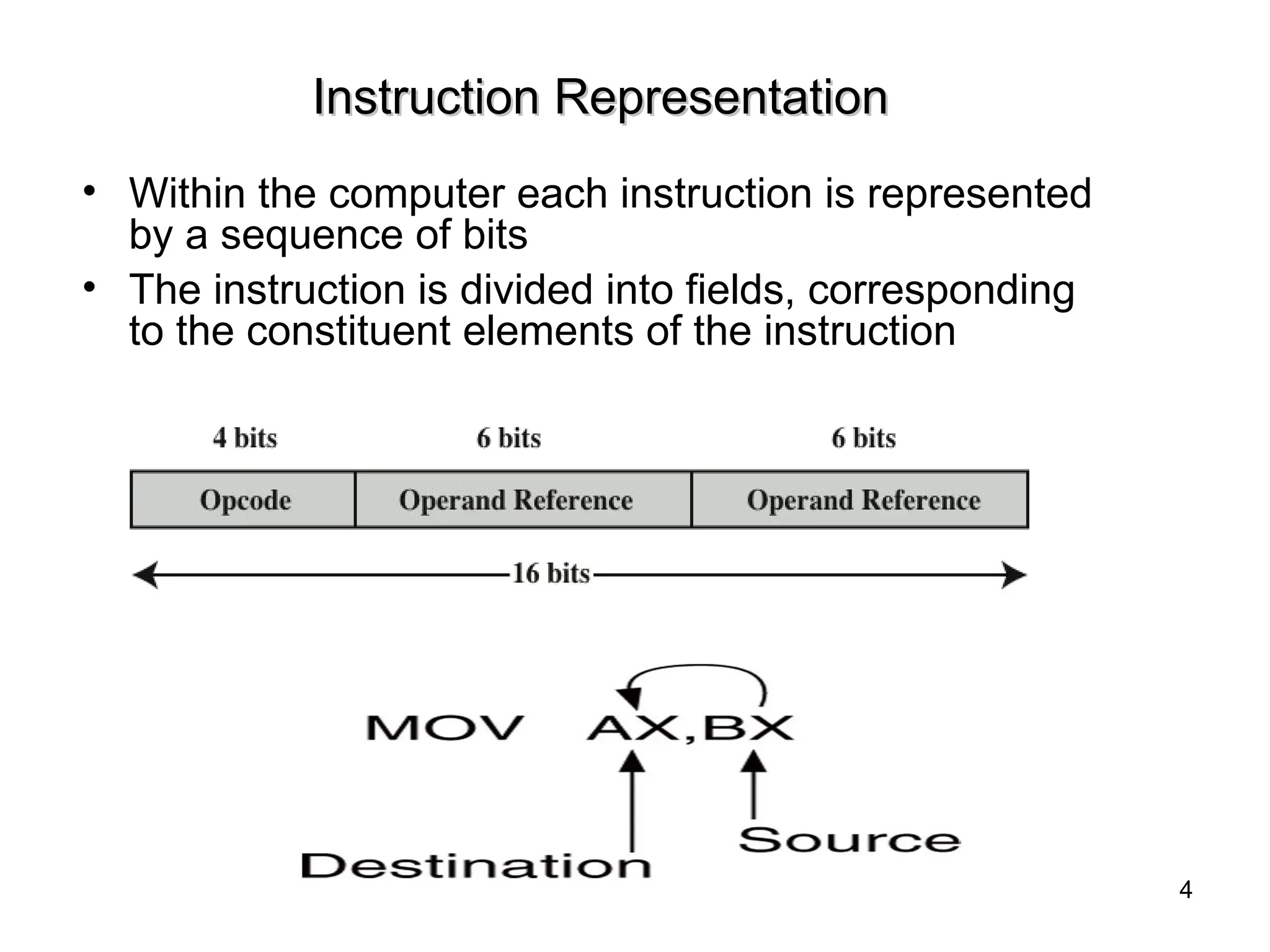
•Within the computer each instruction is represented
by a sequence of bits
• The instruction is divided into fields, corresponding
to the constituent elements of the instruction
4
5.
Instruction Representation…..
Instruction Representation…..
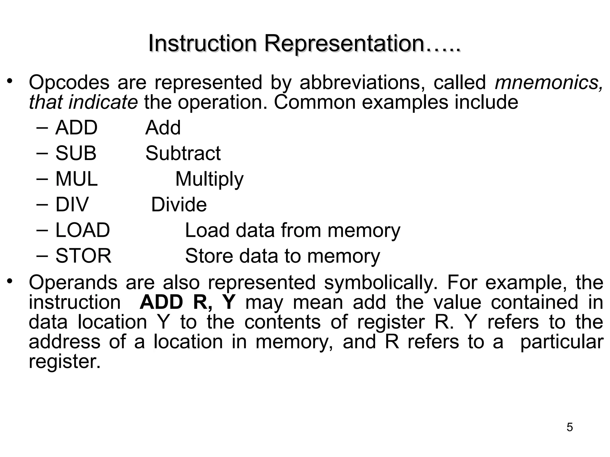
•Opcodes are represented by abbreviations, called mnemonics,
that indicate the operation. Common examples include
– ADD Add
– SUB Subtract
– MUL Multiply
– DIV Divide
– LOAD Load data from memory
– STOR Store data to memory
• Operands are also represented symbolically. For example, the
instruction ADD R, Y may mean add the value contained in
data location Y to the contents of register R. Y refers to the
address of a location in memory, and R refers to a particular
register.
5
6.
Instruction Set Design(1)
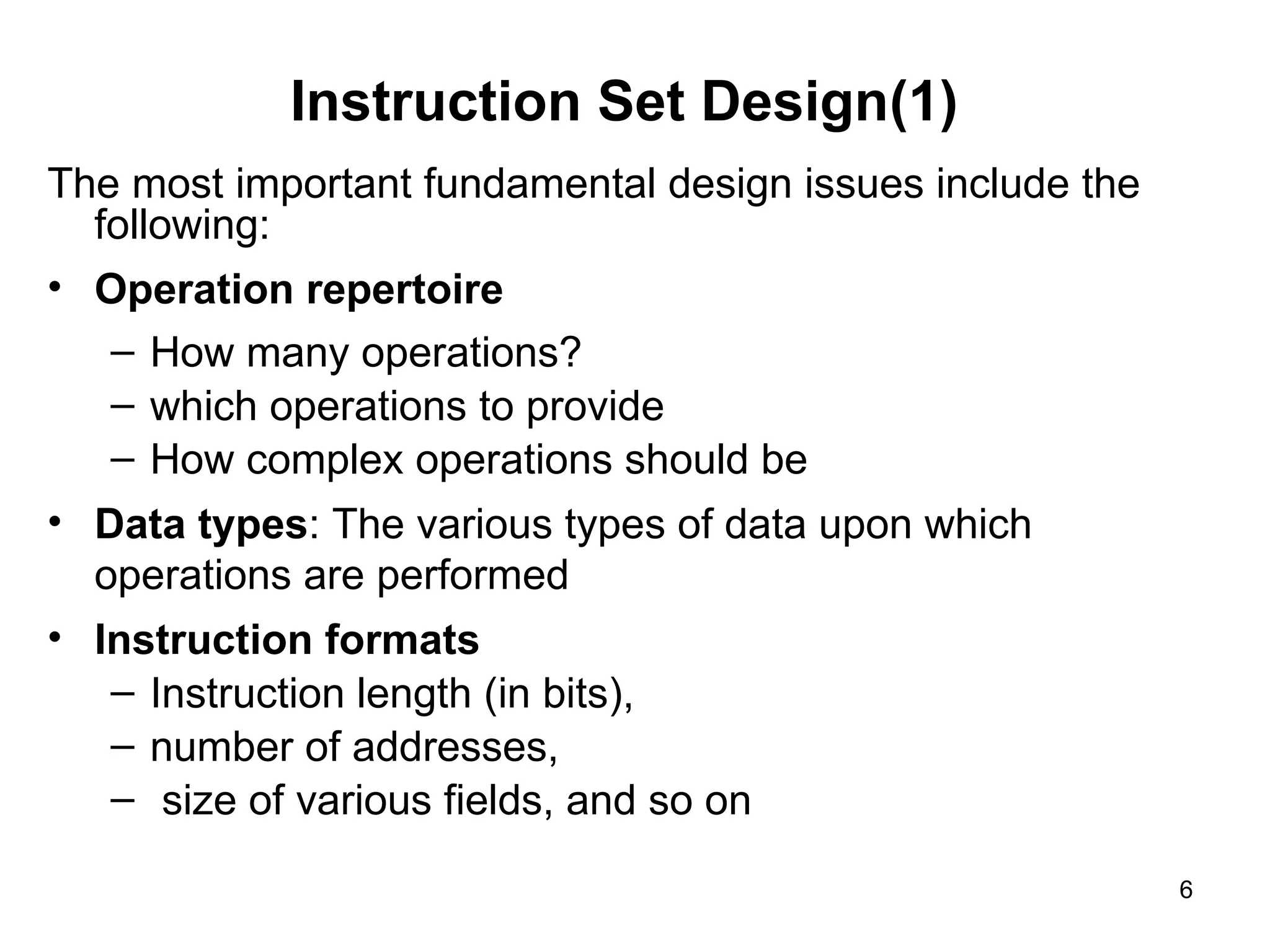
Themost important fundamental design issues include the
following:
• Operation repertoire
– How many operations?
– which operations to provide
– How complex operations should be
• Data types: The various types of data upon which
operations are performed
• Instruction formats
– Instruction length (in bits),
– number of addresses,
– size of various fields, and so on
6
7.
Instruction Set Design(2)
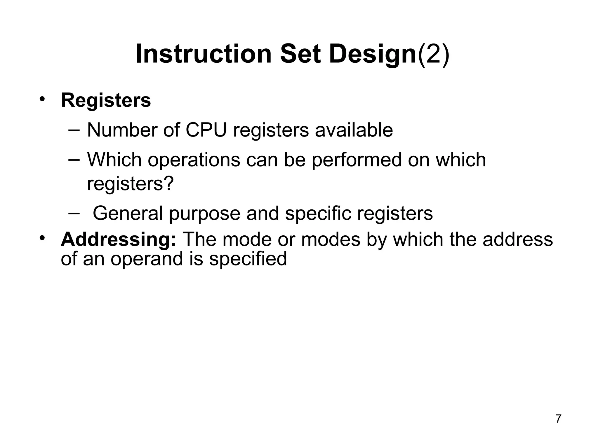
•Registers
– Number of CPU registers available
– Which operations can be performed on which
registers?
– General purpose and specific registers
• Addressing: The mode or modes by which the address
of an operand is specified
7
8.
Instruction Types
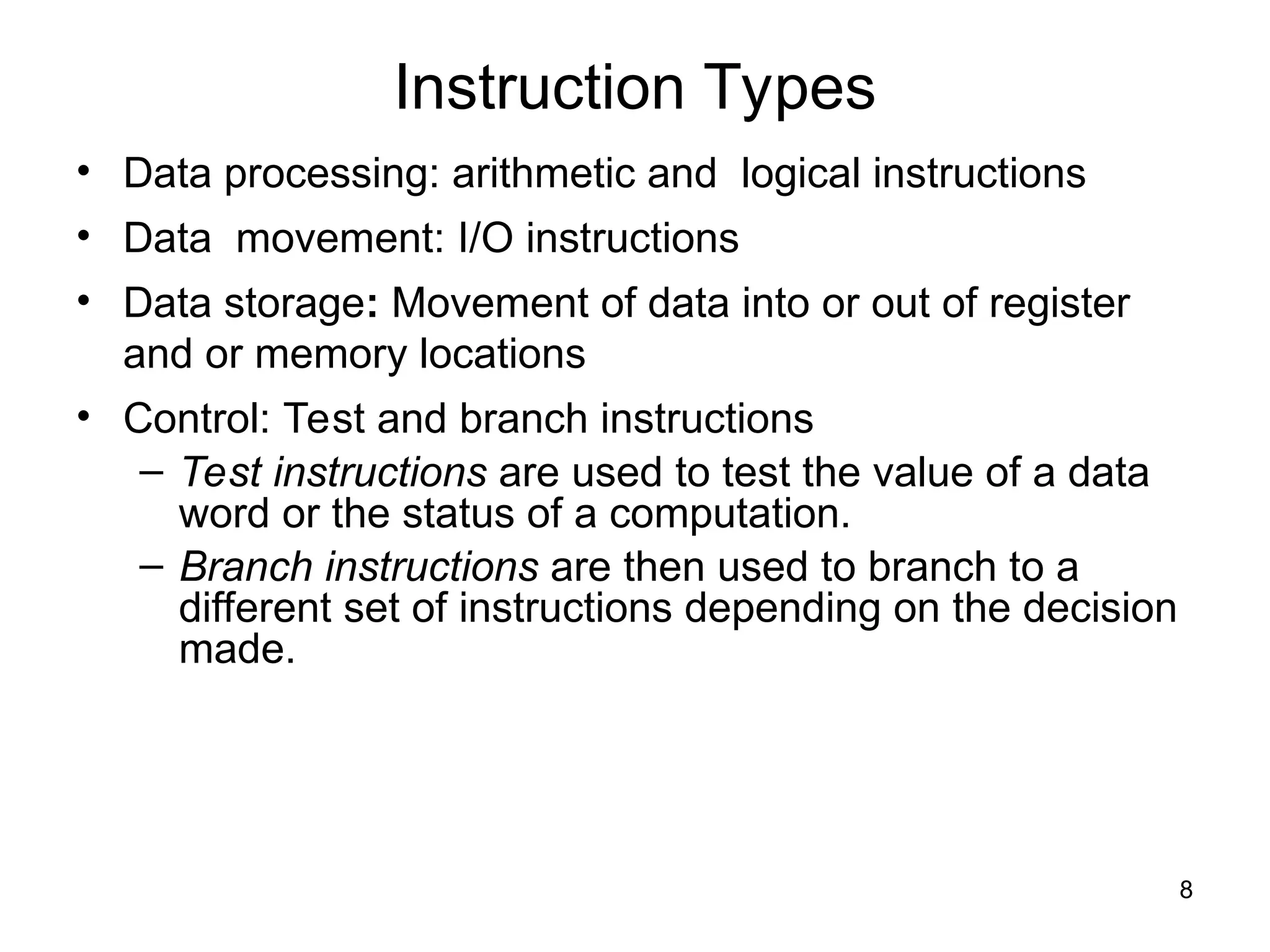
• Dataprocessing: arithmetic and logical instructions
• Data movement: I/O instructions
• Data storage: Movement of data into or out of register
and or memory locations
• Control: Test and branch instructions
– Test instructions are used to test the value of a data
word or the status of a computation.
– Branch instructions are then used to branch to a
different set of instructions depending on the decision
made.
8
9.
Processor Actions forVarious Types of Operations
Processor Actions for Various Types of Operations
9
10.
Types of Operands
•Addresses: addresses are, in fact, a form of data.
addresses can be considered to be unsigned integers.
• Numbers: All machine languages include numeric data
types. Three types of numerical data are common in
computers: Binary integer or binary fixed point , Binary
floating point, decimal.
• Characters: ASCII (128 printable and control characters +
bit for error detection)
• Logical Data: bits or flags, e.g., Boolean 0 and 1
10
11.
Number of Addresses
•More addresses
– More complex (powerful?) instructions
– More registers - inter-register operations are quicker
– Less instructions per program
• Fewer addresses
– Less complex (powerful?) instructions
– More instructions per program, e.g. data movement
– Faster fetch/execution of instructions
• Example: Y=(A-B):[(C+(DxE)]
11
12.
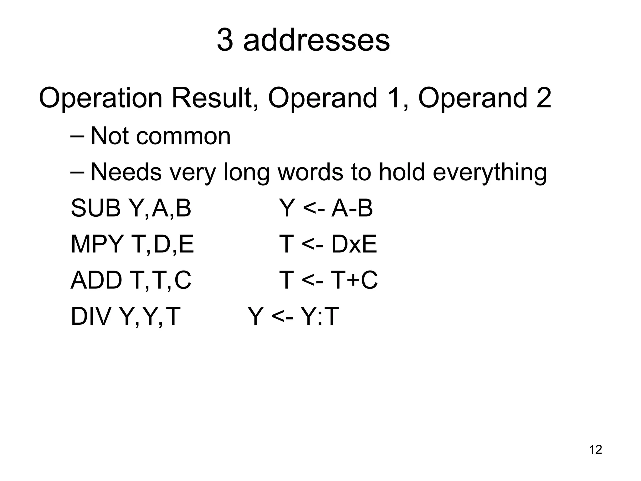
3 addresses
Operation Result,Operand 1, Operand 2
– Not common
– Needs very long words to hold everything
SUB Y,A,B Y <- A-B
MPY T,D,E T <- DxE
ADD T,T,C T <- T+C
DIV Y,Y,T Y <- Y:T
12
13.
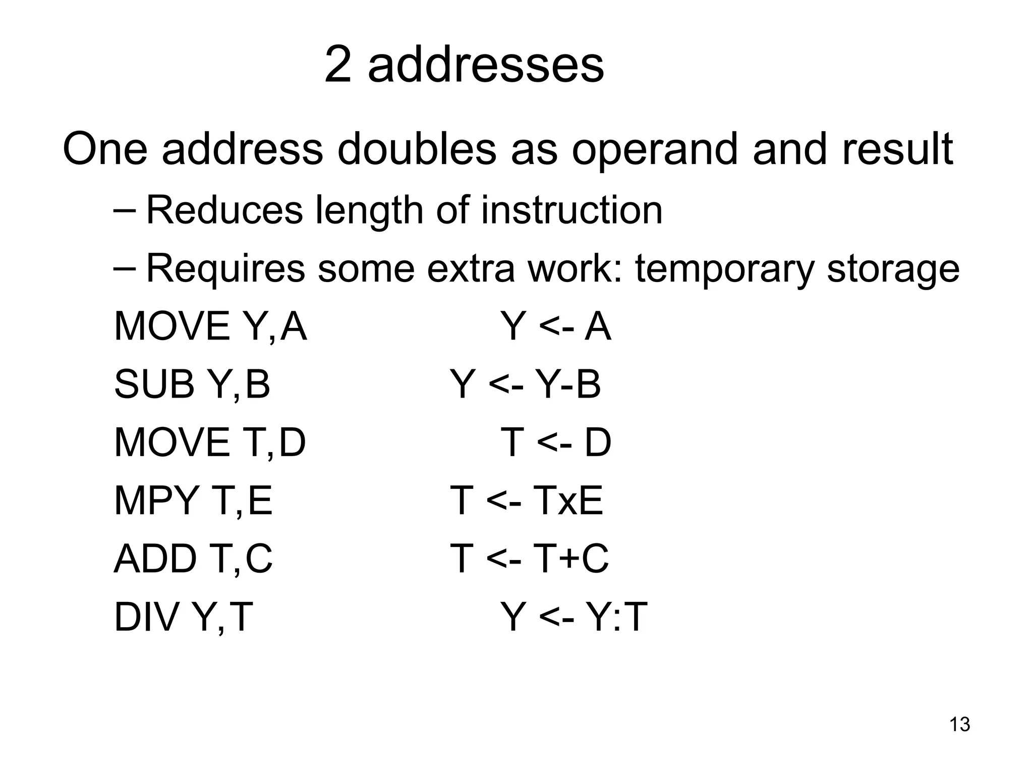
2 addresses
One addressdoubles as operand and result
– Reduces length of instruction
– Requires some extra work: temporary storage
MOVE Y,A Y <- A
SUB Y,B Y <- Y-B
MOVE T,D T <- D
MPY T,E T <- TxE
ADD T,C T <- T+C
DIV Y,T Y <- Y:T
13
14.
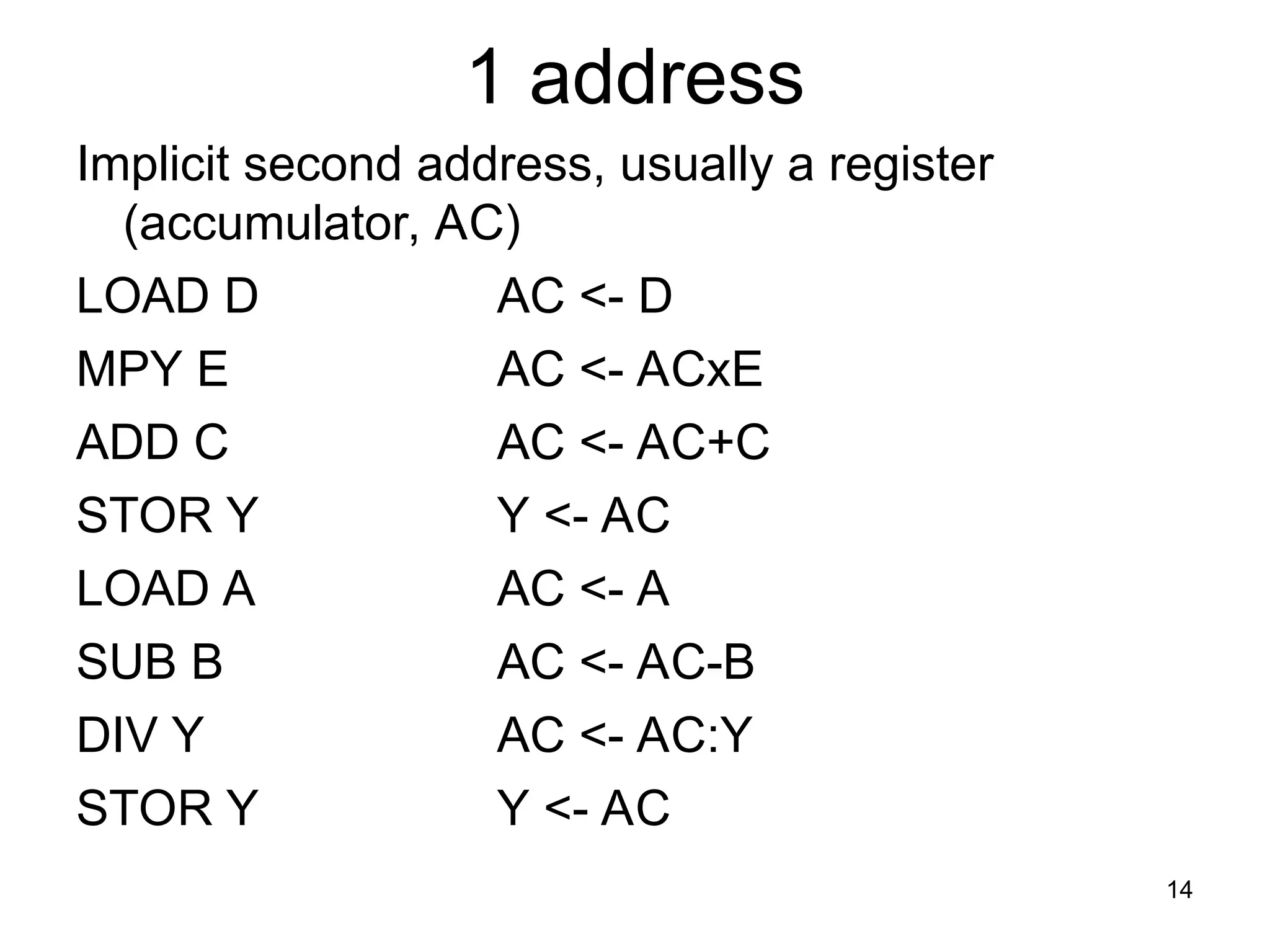
1 address
Implicit secondaddress, usually a register
(accumulator, AC)
LOAD D AC <- D
MPY E AC <- ACxE
ADD C AC <- AC+C
STOR Y Y <- AC
LOAD A AC <- A
SUB B AC <- AC-B
DIV Y AC <- AC:Y
STOR Y Y <- AC
14
15.
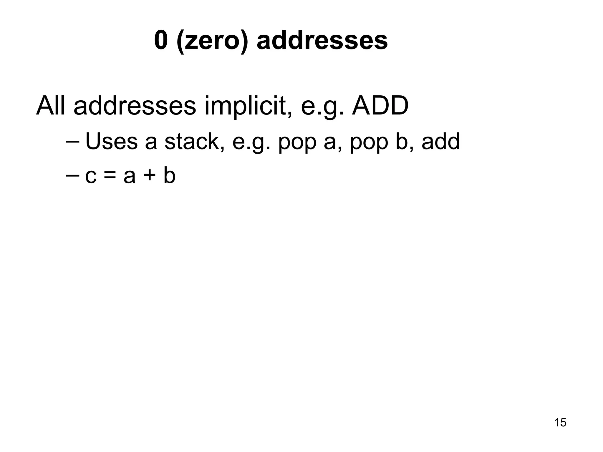
0 (zero) addresses
Alladdresses implicit, e.g. ADD
– Uses a stack, e.g. pop a, pop b, add
– c = a + b
15
16.
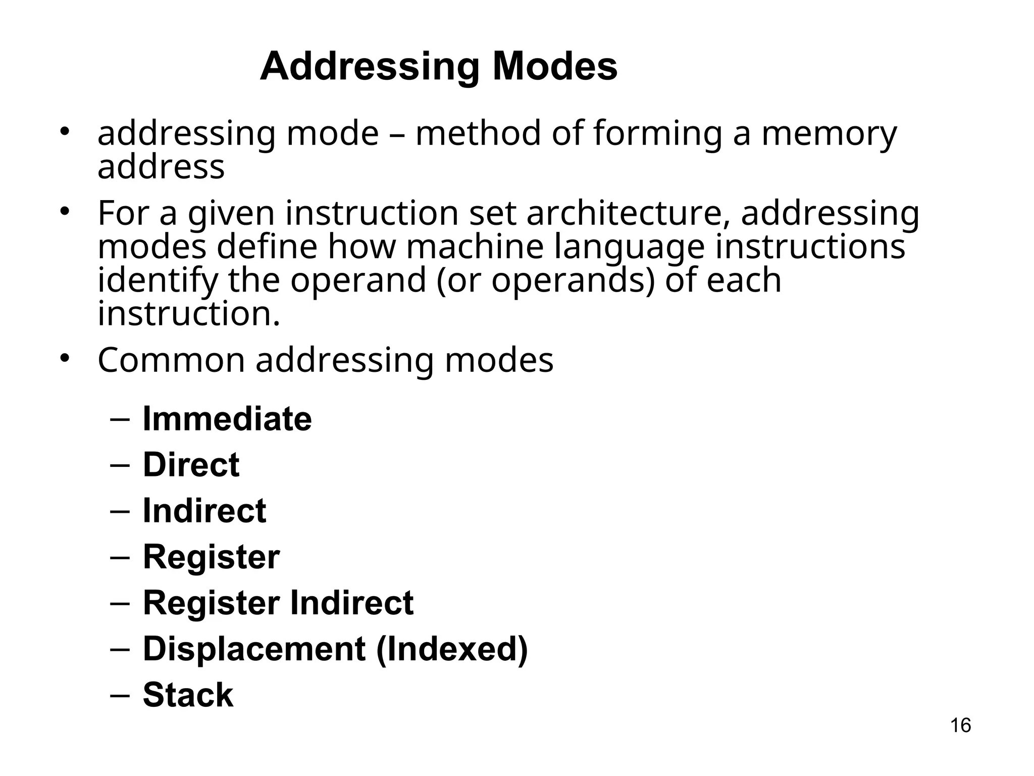
Addressing Modes
• addressingmode – method of forming a memory
address
• For a given instruction set architecture, addressing
modes define how machine language instructions
identify the operand (or operands) of each
instruction.
• Common addressing modes
– Immediate
– Direct
– Indirect
– Register
– Register Indirect
– Displacement (Indexed)
– Stack
16
17.
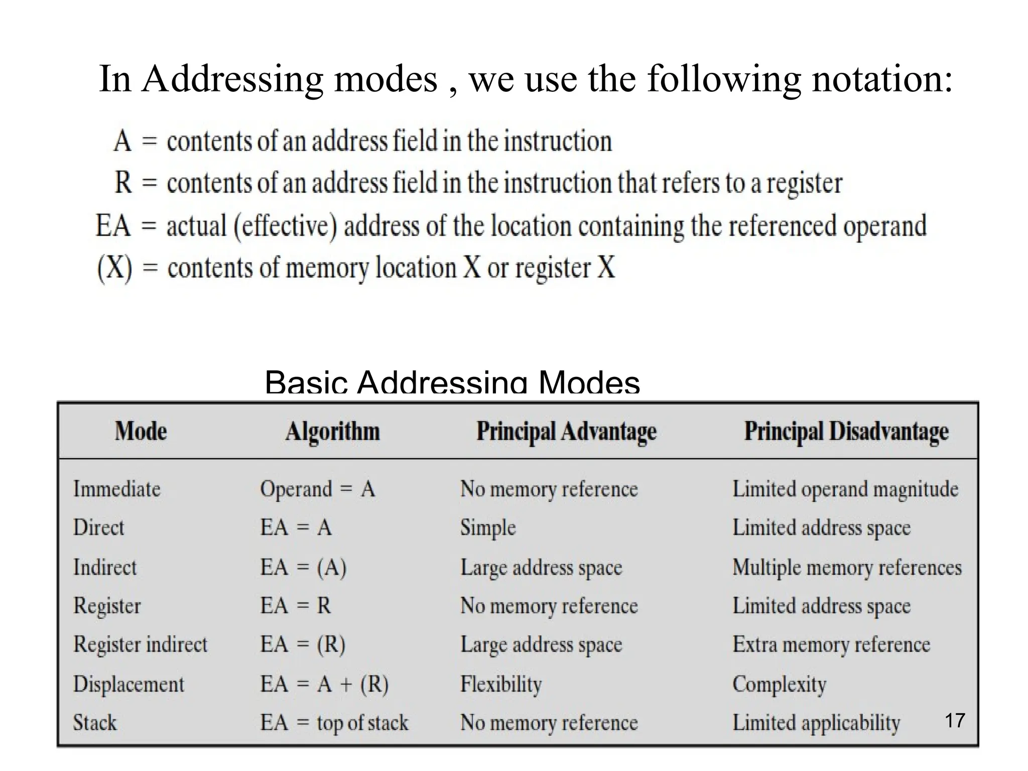
Basic Addressing Modes
weuse the f we use the
In Addressing modes , we use the following notation:
17
18.
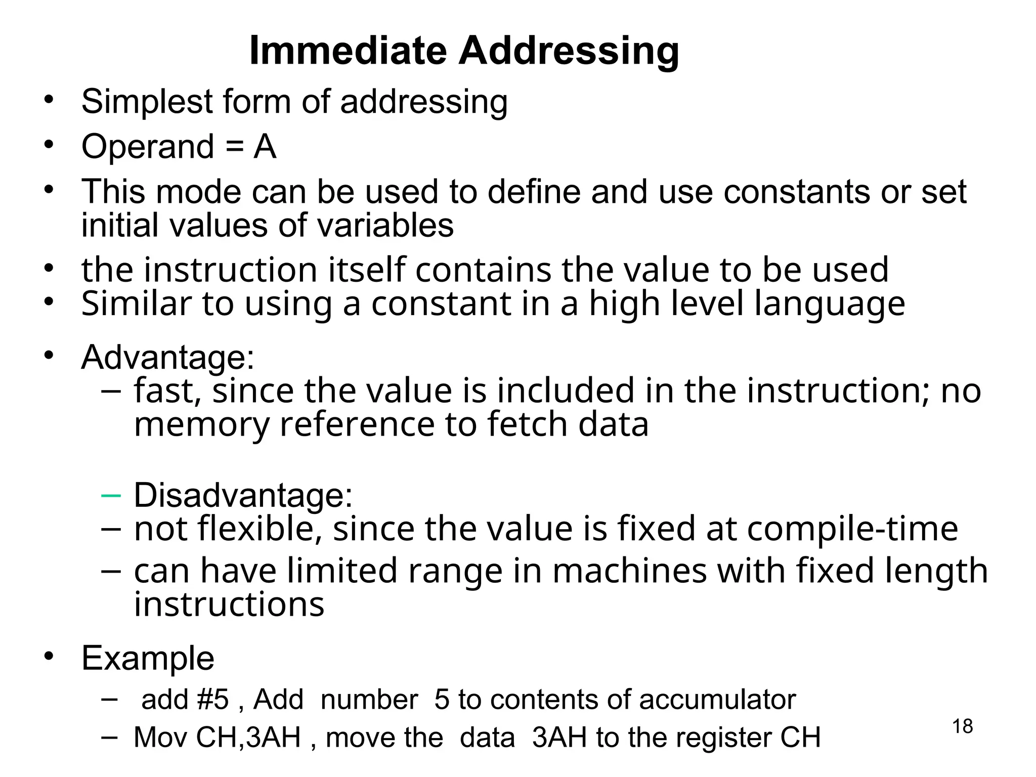
Immediate Addressing
18
• Simplestform of addressing
• Operand = A
• This mode can be used to define and use constants or set
initial values of variables
• the instruction itself contains the value to be used
• Similar to using a constant in a high level language
• Advantage:
– fast, since the value is included in the instruction; no
memory reference to fetch data
– Disadvantage:
– not flexible, since the value is fixed at compile-time
– can have limited range in machines with fixed length
instructions
• Example
– add #5 , Add number 5 to contents of accumulator
– Mov CH,3AH , move the data 3AH to the register CH
19.
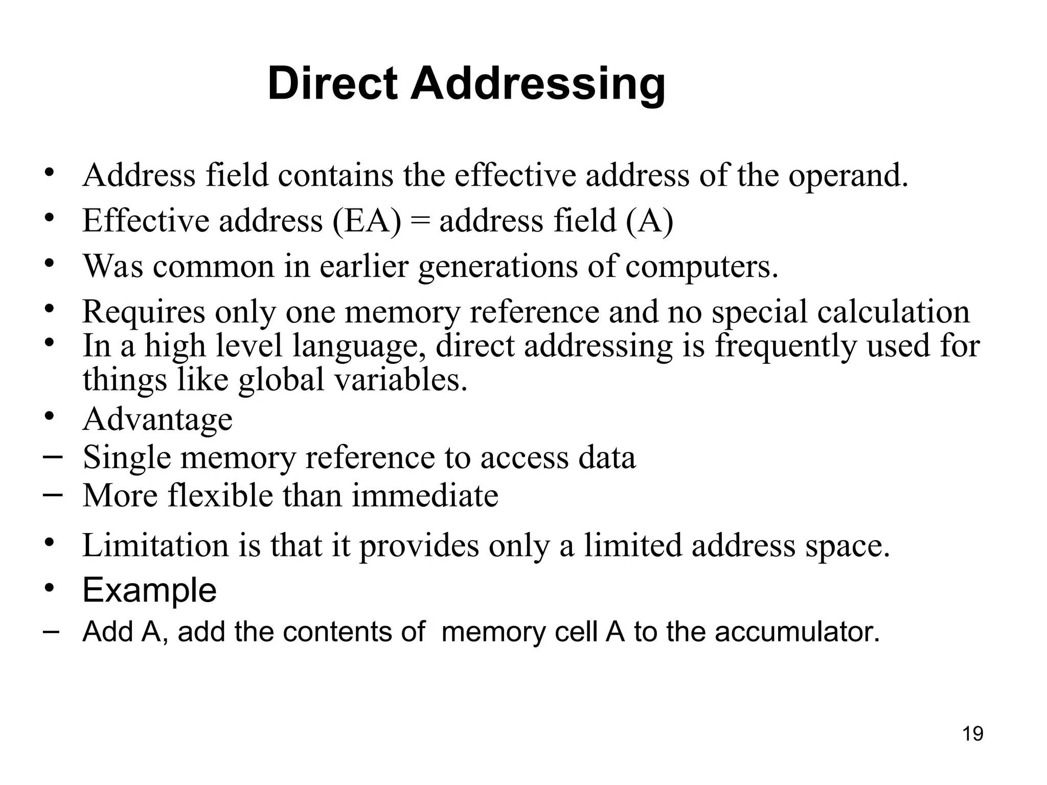
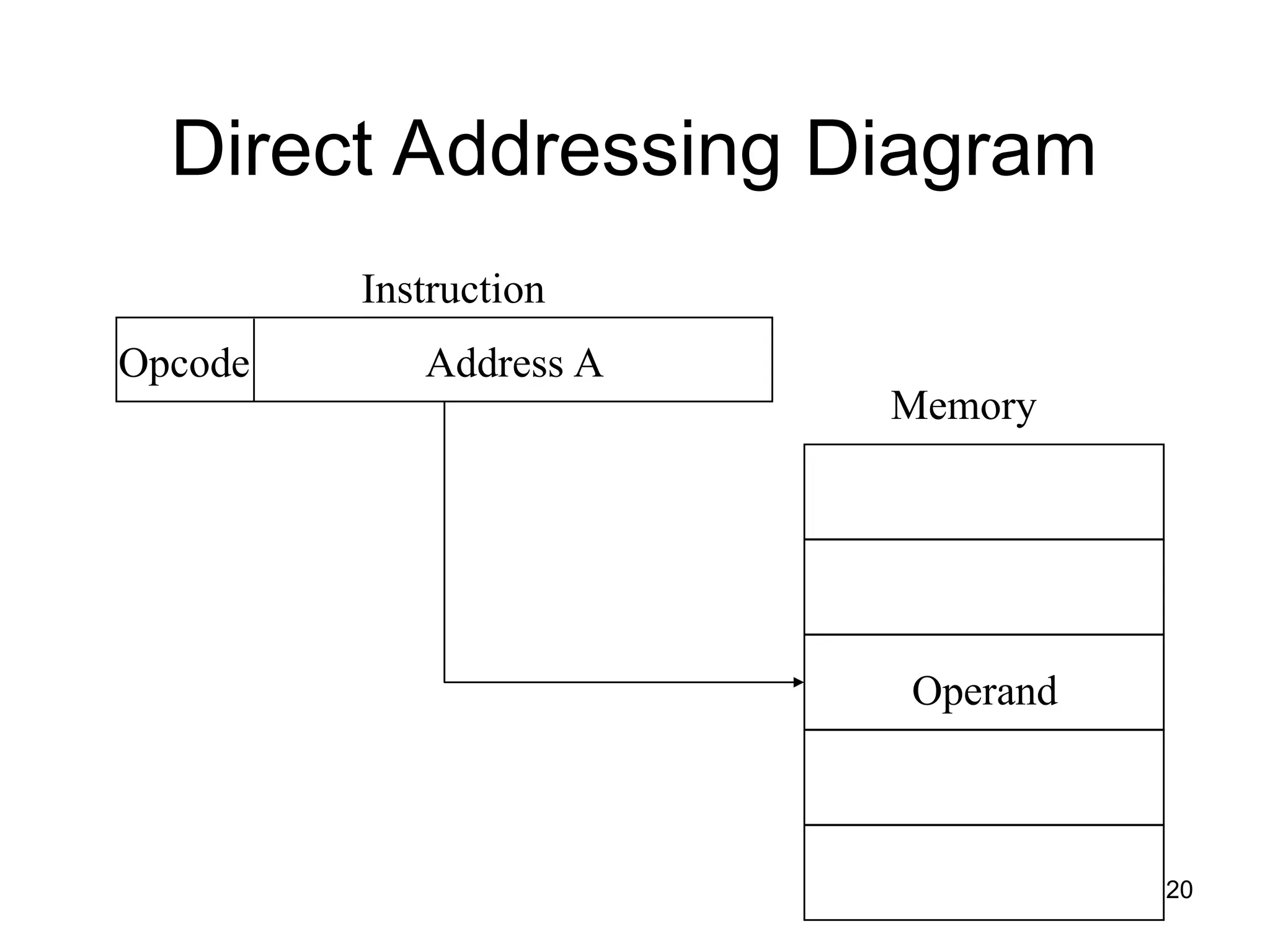
Direct Addressing
• Addressfield contains the effective address of the operand.
• Effective address (EA) = address field (A)
• Was common in earlier generations of computers.
• Requires only one memory reference and no special calculation
• In a high level language, direct addressing is frequently used for
things like global variables.
• Advantage
– Single memory reference to access data
– More flexible than immediate
• Limitation is that it provides only a limited address space.
• Example
– Add A, add the contents of memory cell A to the accumulator.
19
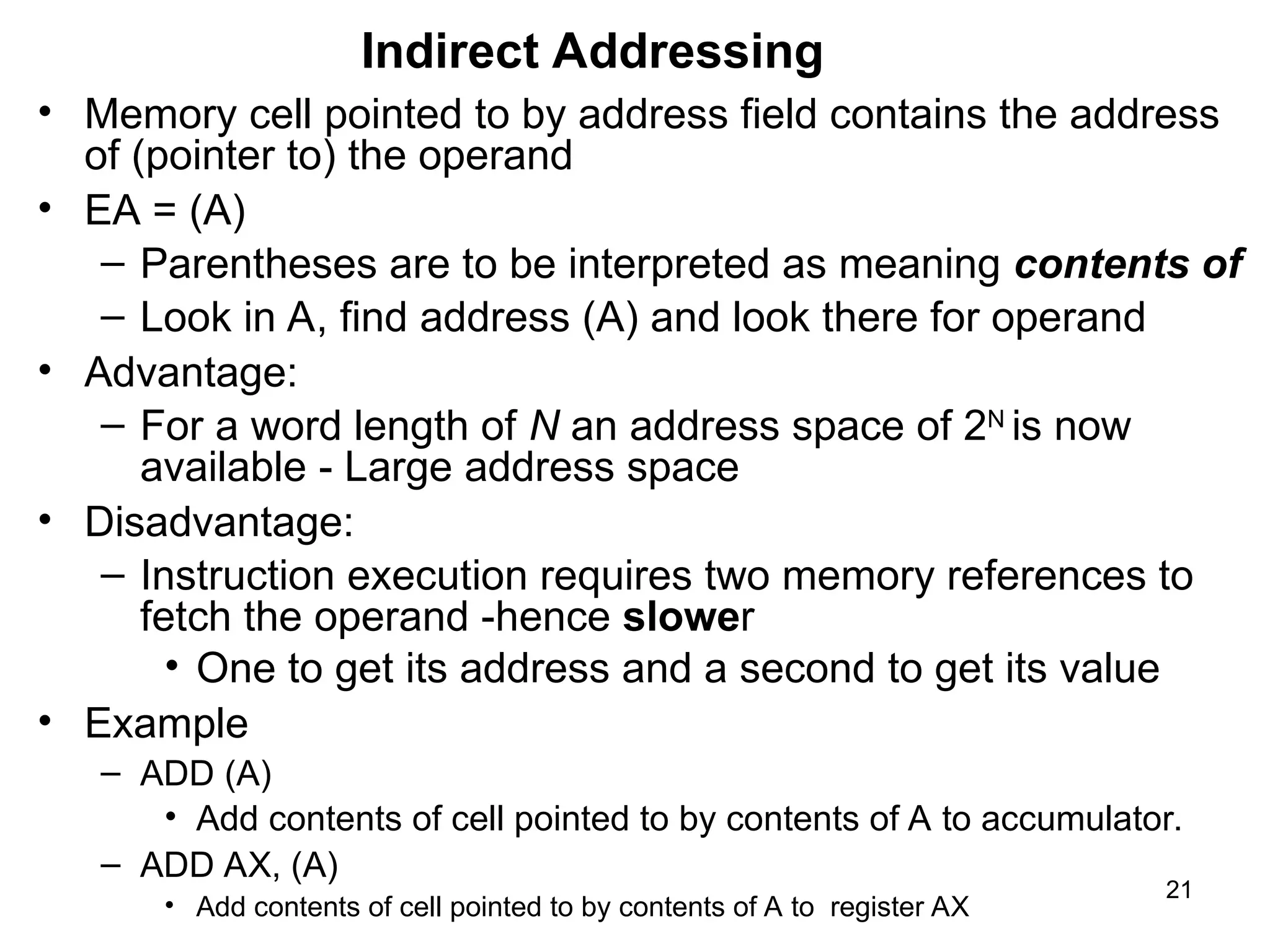
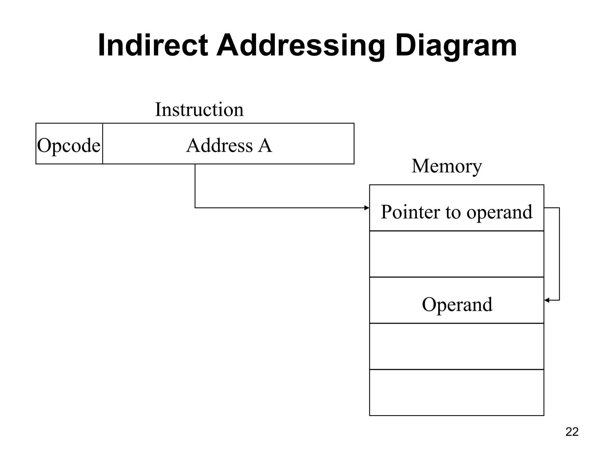
Indirect Addressing
• Memorycell pointed to by address field contains the address
of (pointer to) the operand
• EA = (A)
– Parentheses are to be interpreted as meaning contents of
– Look in A, find address (A) and look there for operand
• Advantage:
– For a word length of N an address space of 2N
is now
available - Large address space
• Disadvantage:
– Instruction execution requires two memory references to
fetch the operand -hence slower
• One to get its address and a second to get its value
• Example
– ADD (A)
• Add contents of cell pointed to by contents of A to accumulator.
– ADD AX, (A)
• Add contents of cell pointed to by contents of A to register AX
21
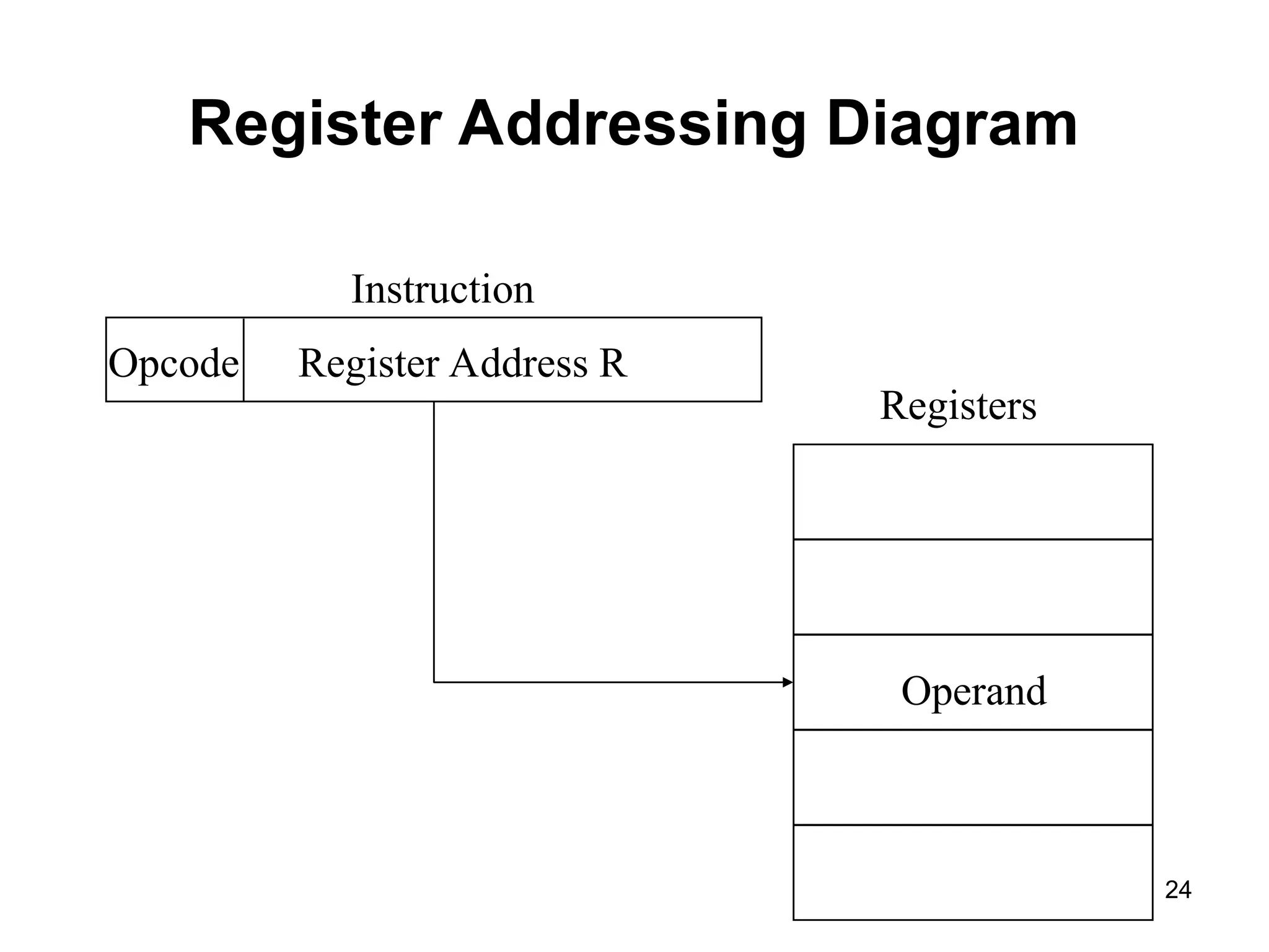
Register Addressing
• Addressfield refers to a register rather than a
main memory address
• EA = R
• Advantages:
– Only a small address field is needed in the instruction
– No time-consuming memory references are required
• Disadvantage:
– The address space is very limited
• Example
– MOV AX, BX
– ADD AX, BX
23
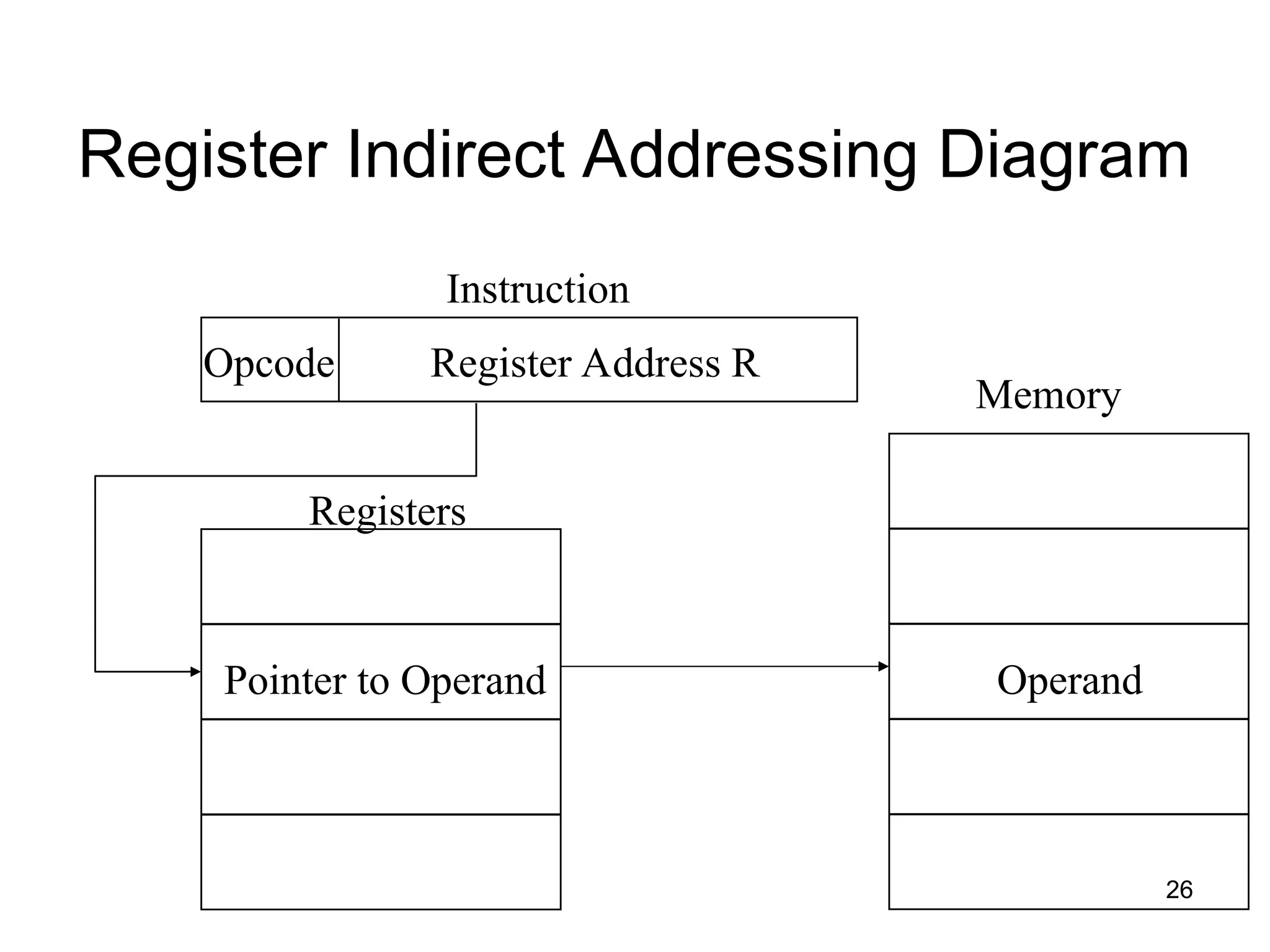
Register Indirect Addressing
•Analogous to indirect addressing
– The only difference is whether the address field
refers to a memory location or a register
• EA = (R)
• Address space limitation of the address field is
overcome by having that field refer to a word-length
location containing an address
• Uses one less memory reference than indirect
addressing
• Example
– ADD (R)
25
26.
Register Indirect AddressingDiagram
Register Address R
Opcode
Instruction
Memory
Operand
Pointer to Operand
Registers
26
27.
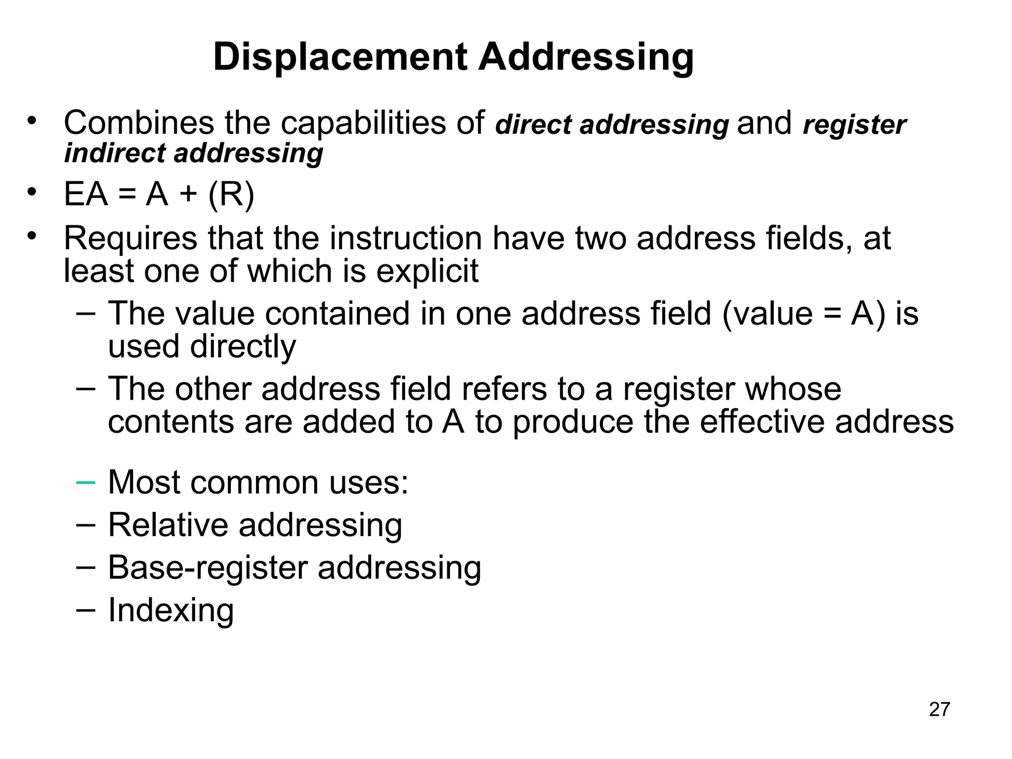
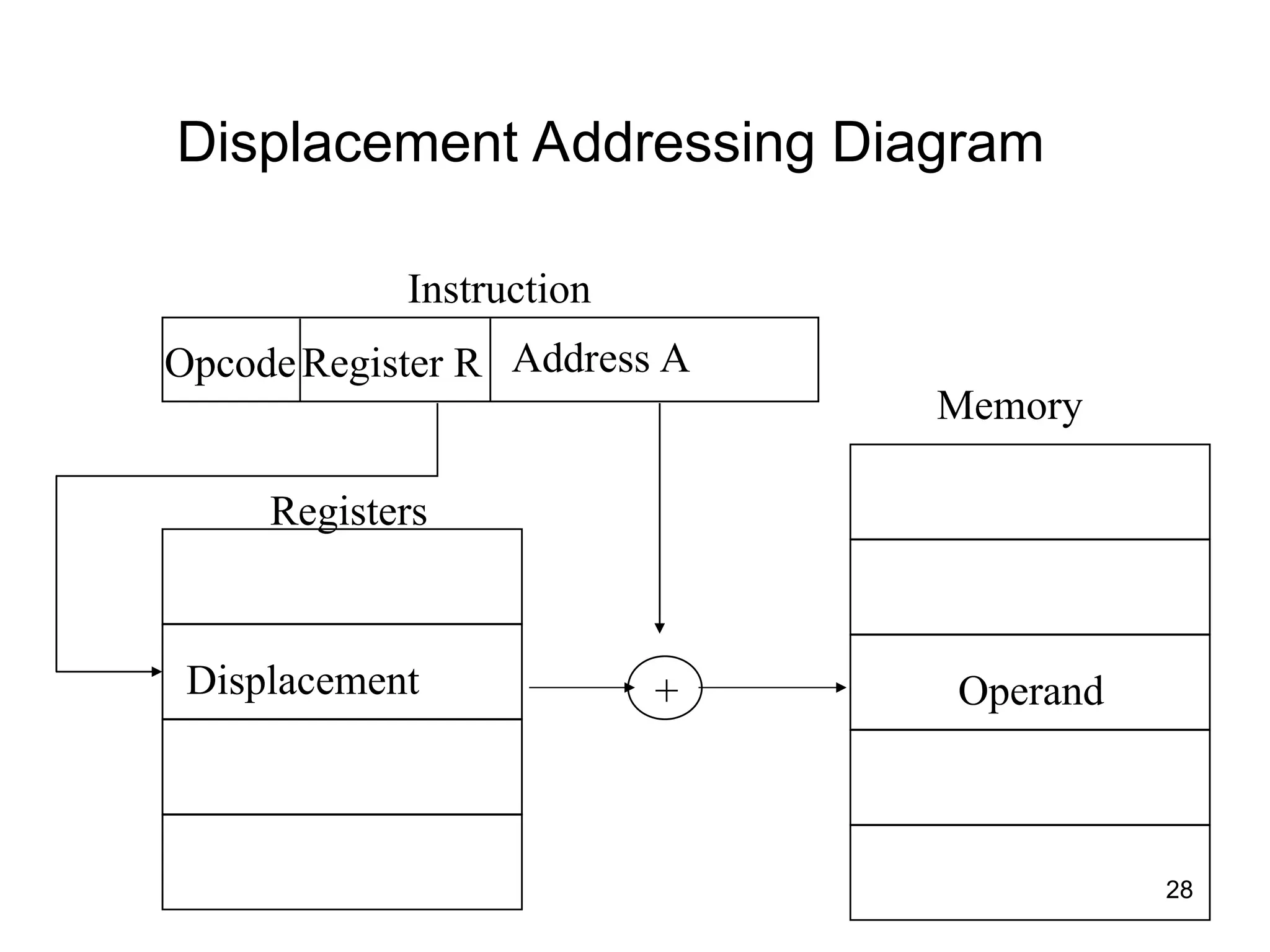
Displacement Addressing
• Combinesthe capabilities of direct addressing and register
indirect addressing
• EA = A + (R)
• Requires that the instruction have two address fields, at
least one of which is explicit
– The value contained in one address field (value = A) is
used directly
– The other address field refers to a register whose
contents are added to A to produce the effective address
– Most common uses:
– Relative addressing
– Base-register addressing
– Indexing
27
Relative Addressing
• EA= A + (PC)
• Address field A is treated as 2’s complement integer to
allow backward references
• Fetch operand from PC+A
• Can be very efficient because of locality of reference &
cache usage
– But in large programs code and data may be widely
separated in memory
29
30.
Base-Register Addressing
Base-Register Addressing
•A holds displacement
• R holds pointer to base address
• R may be explicit or implicit
– E.g. segment registers in 80x86 are base
registers and are involved in all EA computations
– X86 processors have a wide variety of base
addressing
30
31.
Indexed addressing
• A= Base
• R = displacement
• EA = A + R
• Good for accessing arrays
– EA = A + R
– R++
• Iterative access to sequential memory locations is
very common
• Some architectures provide auto-increment or auto-
decrement
• Pre index EA = A + (R++)
• Post index EA = A + (++R)
• The ARM architecture provides pre indexed and post
indexed addressing 31
32.
Stack Addressing
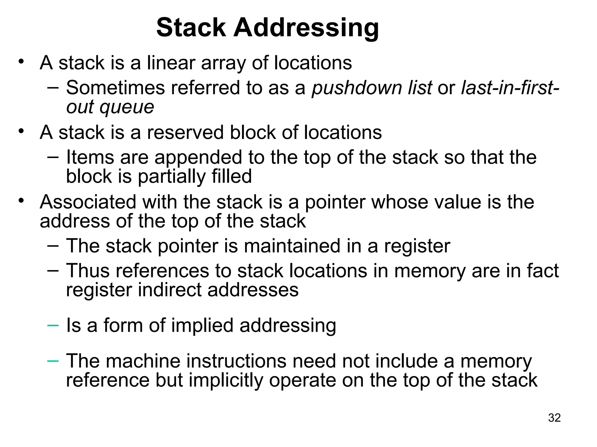
• Astack is a linear array of locations
– Sometimes referred to as a pushdown list or last-in-first-
out queue
• A stack is a reserved block of locations
– Items are appended to the top of the stack so that the
block is partially filled
• Associated with the stack is a pointer whose value is the
address of the top of the stack
– The stack pointer is maintained in a register
– Thus references to stack locations in memory are in fact
register indirect addresses
– Is a form of implied addressing
– The machine instructions need not include a memory
reference but implicitly operate on the top of the stack
32
33.
Processor Organization
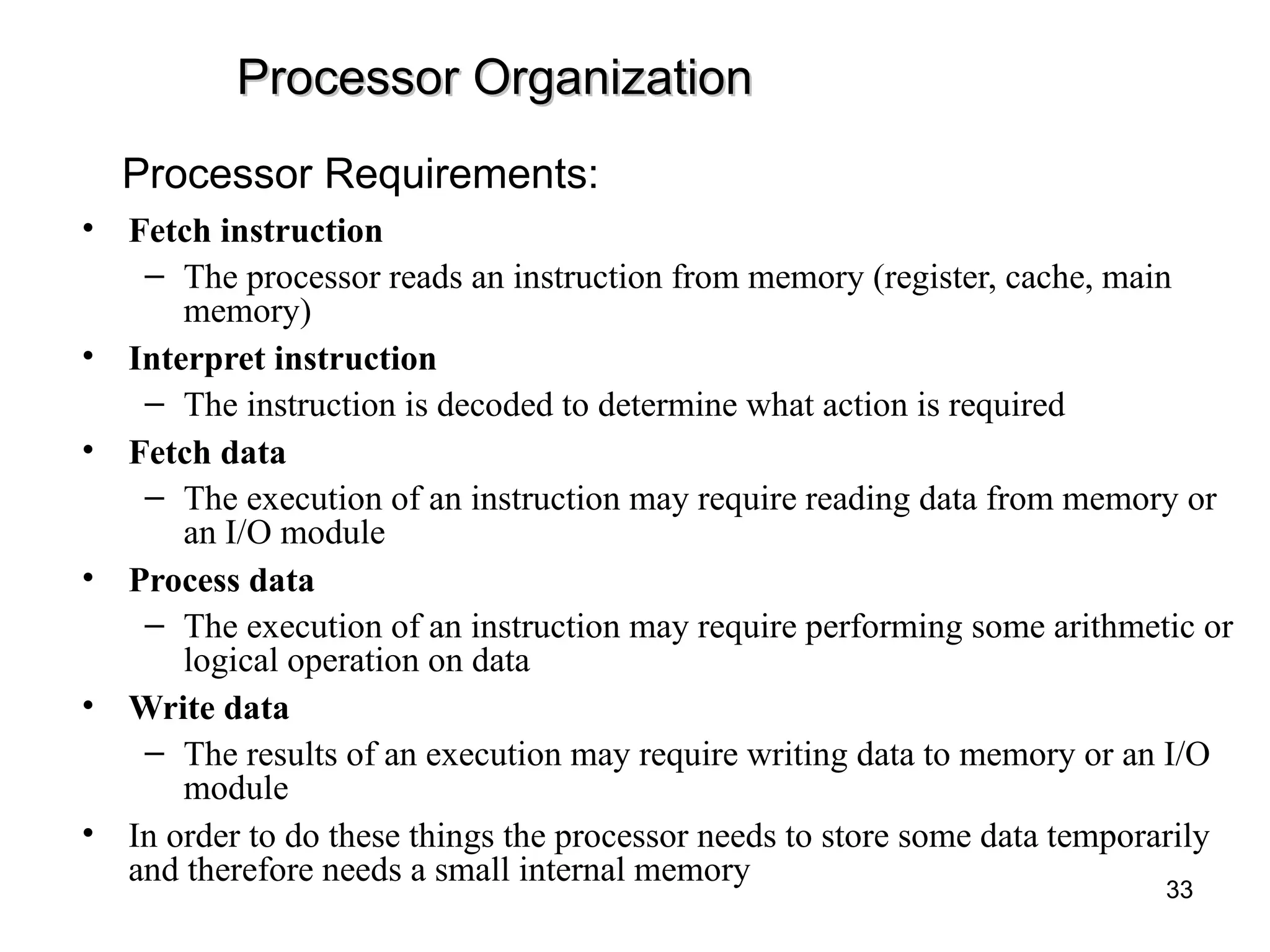
Processor Organization
•Fetch instruction
– The processor reads an instruction from memory (register, cache, main
memory)
• Interpret instruction
– The instruction is decoded to determine what action is required
• Fetch data
– The execution of an instruction may require reading data from memory or
an I/O module
• Process data
– The execution of an instruction may require performing some arithmetic or
logical operation on data
• Write data
– The results of an execution may require writing data to memory or an I/O
module
• In order to do these things the processor needs to store some data temporarily
and therefore needs a small internal memory
Processor Requirements:
33
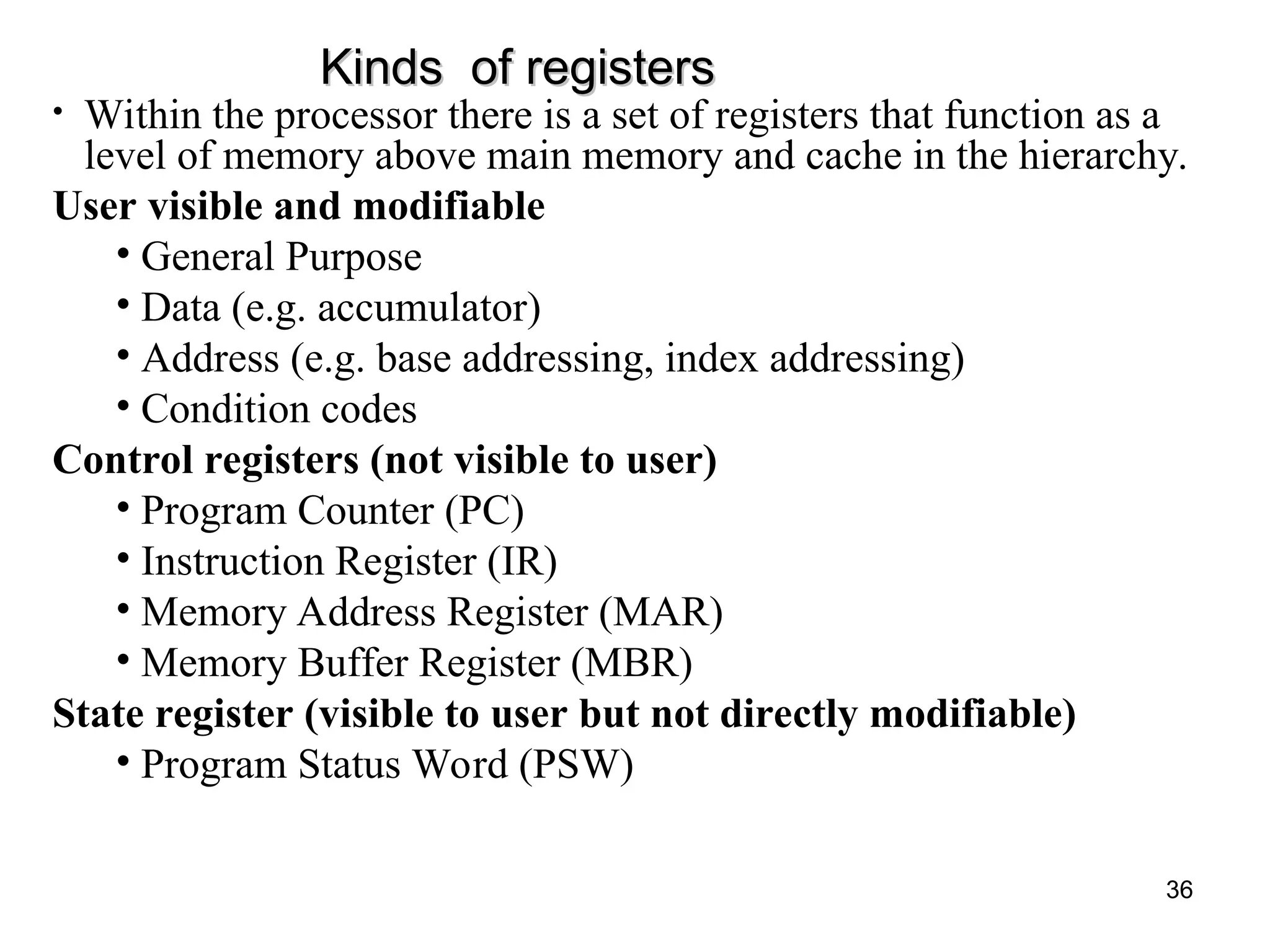
Kinds of registers
Kindsof registers
• Within the processor there is a set of registers that function as a
level of memory above main memory and cache in the hierarchy.
User visible and modifiable
• General Purpose
• Data (e.g. accumulator)
• Address (e.g. base addressing, index addressing)
• Condition codes
Control registers (not visible to user)
• Program Counter (PC)
• Instruction Register (IR)
• Memory Address Register (MAR)
• Memory Buffer Register (MBR)
State register (visible to user but not directly modifiable)
• Program Status Word (PSW)
36
37.
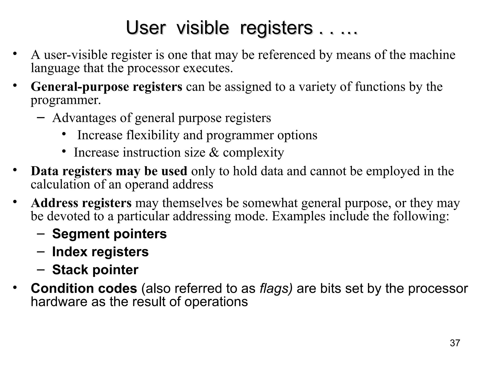
User visible registers. . …
User visible registers . . …
• A user-visible register is one that may be referenced by means of the machine
language that the processor executes.
• General-purpose registers can be assigned to a variety of functions by the
programmer.
– Advantages of general purpose registers
• Increase flexibility and programmer options
• Increase instruction size & complexity
• Data registers may be used only to hold data and cannot be employed in the
calculation of an operand address
• Address registers may themselves be somewhat general purpose, or they may
be devoted to a particular addressing mode. Examples include the following:
– Segment pointers
– Index registers
– Stack pointer
• Condition codes (also referred to as flags) are bits set by the processor
hardware as the result of operations
37
38.
Control Registers
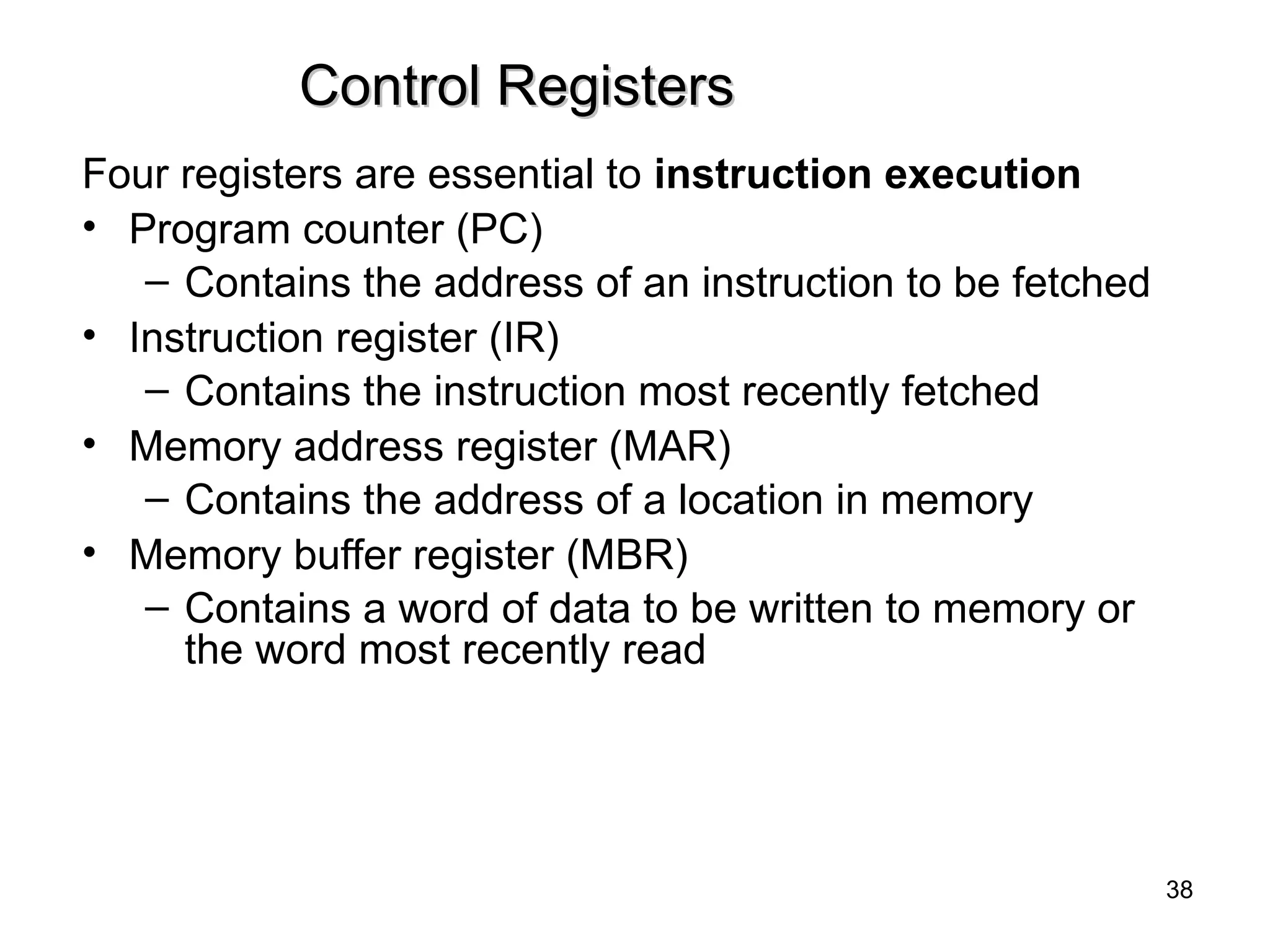
Control Registers
Fourregisters are essential to instruction execution
• Program counter (PC)
– Contains the address of an instruction to be fetched
• Instruction register (IR)
– Contains the instruction most recently fetched
• Memory address register (MAR)
– Contains the address of a location in memory
• Memory buffer register (MBR)
– Contains a word of data to be written to memory or
the word most recently read
38
39.
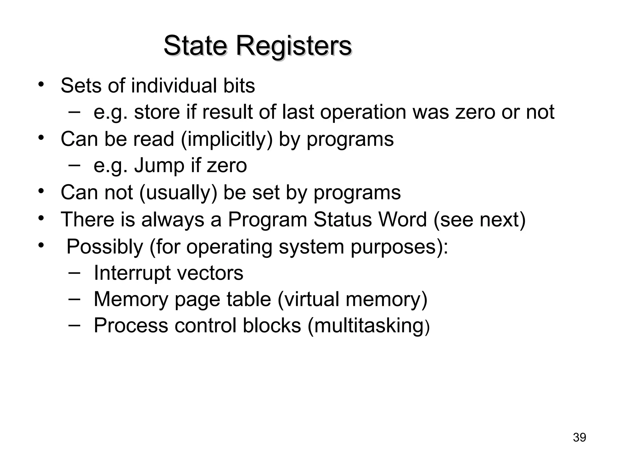
State Registers
State Registers
•Sets of individual bits
– e.g. store if result of last operation was zero or not
• Can be read (implicitly) by programs
– e.g. Jump if zero
• Can not (usually) be set by programs
• There is always a Program Status Word (see next)
• Possibly (for operating system purposes):
– Interrupt vectors
– Memory page table (virtual memory)
– Process control blocks (multitasking)
39
40.
Program Status Word(PSW)
Program Status Word (PSW)
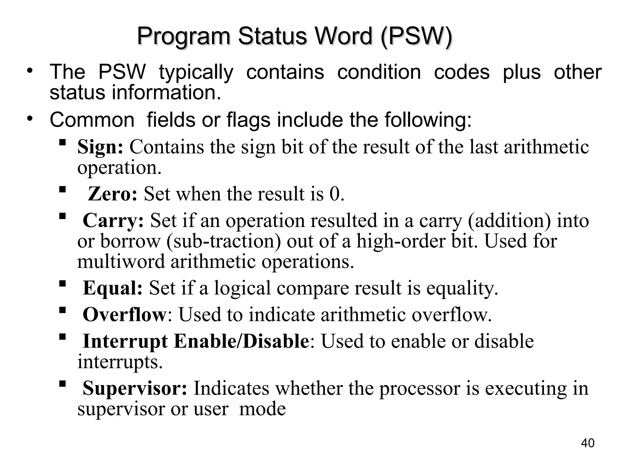
• The PSW typically contains condition codes plus other
status information.
• Common fields or flags include the following:
Sign: Contains the sign bit of the result of the last arithmetic
operation.
Zero: Set when the result is 0.
Carry: Set if an operation resulted in a carry (addition) into
or borrow (sub-traction) out of a high-order bit. Used for
multiword arithmetic operations.
Equal: Set if a logical compare result is equality.
Overflow: Used to indicate arithmetic overflow.
Interrupt Enable/Disable: Used to enable or disable
interrupts.
Supervisor: Indicates whether the processor is executing in
supervisor or user mode
40
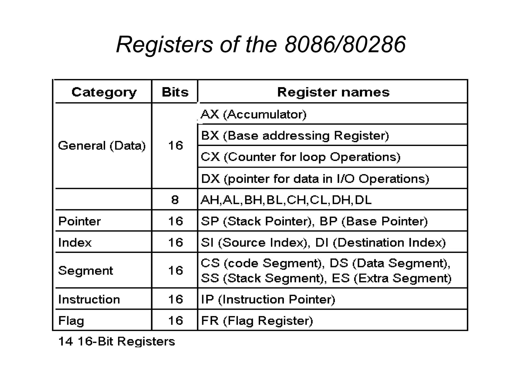
General Purpose Registers
GeneralPurpose Registers
• AX (Accumulator) – favored by CPU for arithmetic
operations
• BX – Base – can hold the address of a procedure or
variable (SI, DI, and BP can also).
– Can also perform arithmetic and data movement.
• CX – acts as a counter for repeating or looping
instructions.
• DX – holds the high 16 bits of the product in multiply
(also handles divide operations)
44.
Segment Registers
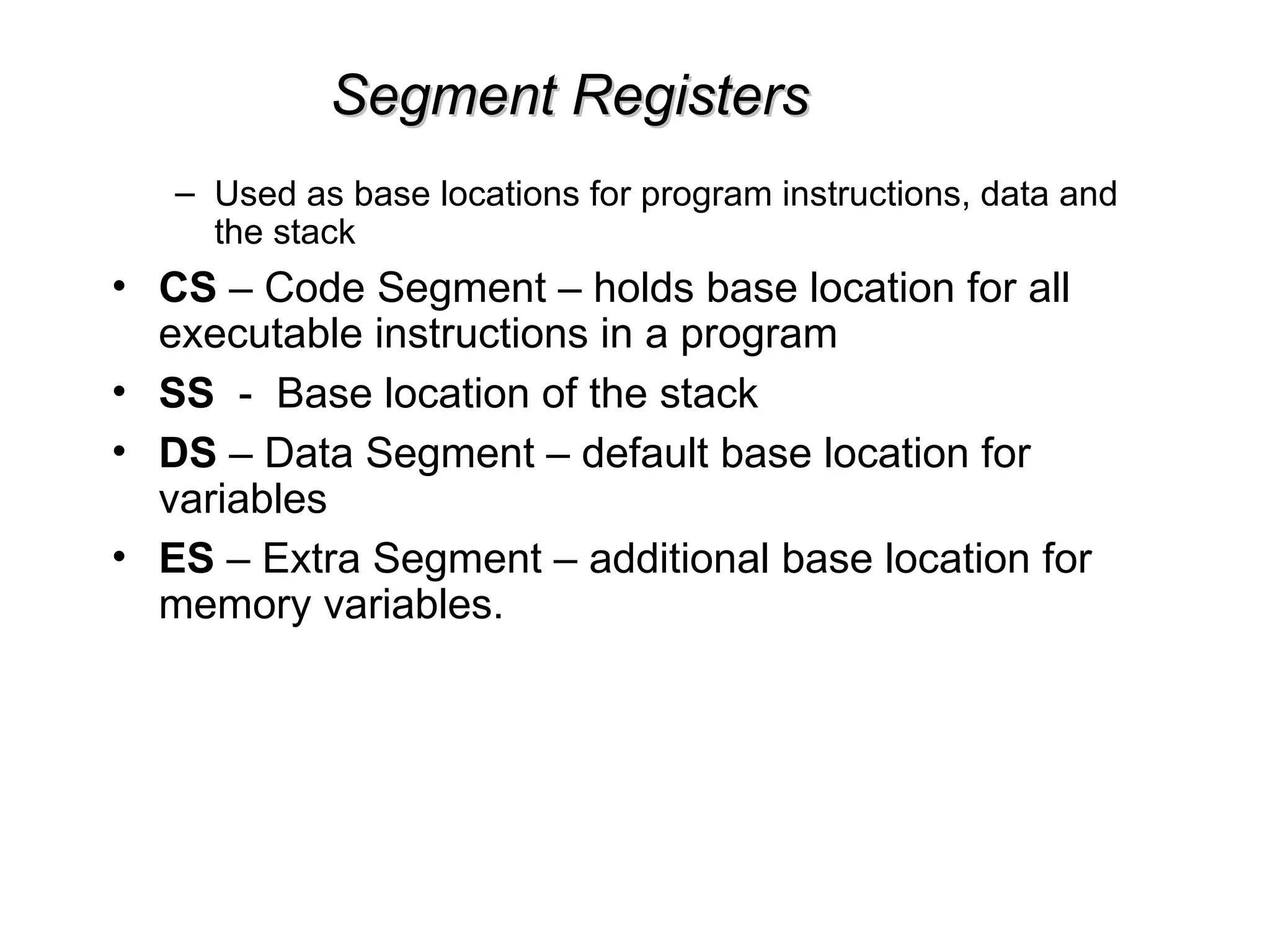
Segment Registers
–Used as base locations for program instructions, data and
the stack
• CS – Code Segment – holds base location for all
executable instructions in a program
• SS - Base location of the stack
• DS – Data Segment – default base location for
variables
• ES – Extra Segment – additional base location for
memory variables.
45.
Pointer Registers
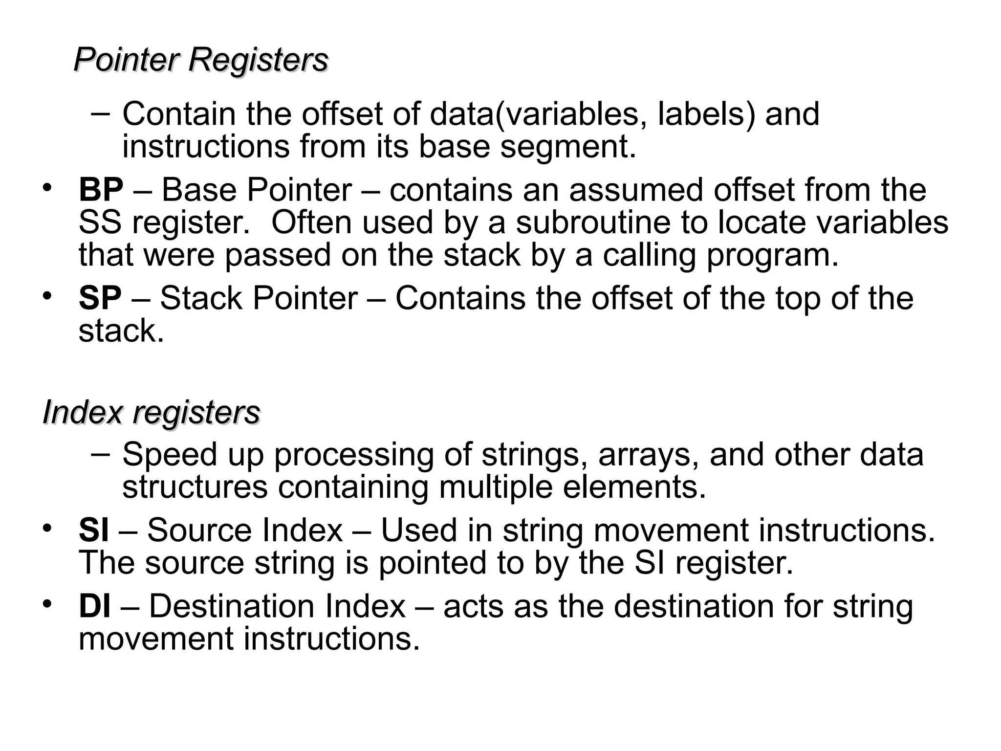
Pointer Registers
–Contain the offset of data(variables, labels) and
instructions from its base segment.
• BP – Base Pointer – contains an assumed offset from the
SS register. Often used by a subroutine to locate variables
that were passed on the stack by a calling program.
• SP – Stack Pointer – Contains the offset of the top of the
stack.
Index registers
Index registers
– Speed up processing of strings, arrays, and other data
structures containing multiple elements.
• SI – Source Index – Used in string movement instructions.
The source string is pointed to by the SI register.
• DI – Destination Index – acts as the destination for string
movement instructions.
Editor's Notes
#2 The operation of the processor is determined by the instructions it executes, referred to as machine instructions or computer instructions. The collection of different instructions that the processor can execute is referred to as the processor’s instruction set.
Each instruction must contain the information required by the processor for execution.
#3 • Operation code: Specifies the operation to be performed (e.g., ADD, I/O). The operation is specified by a binary code, known as the operation code, or opcode.
• Source operand reference: The operation may involve one or more source operands, that is, operands that are inputs for the operation.
• Result operand reference: The operation may produce a result.
• Next instruction reference: This tells the processor where to fetch the next instruction after the execution of this instruction is complete.
#4 Within the computer, each instruction is represented by a sequence of bits. The instruction is divided into fields, corresponding to the constituent elements of the instruction.
A simple example of an instruction format is shown in Figure 12.2. As another example, the IAS instruction format is shown in Figure 2.2. With most instruction sets, more than one format is used. During instruction execution, an instruction is read into an instruction register (IR) in the processor. The processor must be able to extract the data from the various instruction fields to perform the required operation.
It is difficult for both the programmer and the reader of textbooks to deal with binary representations of machine instructions. Thus, it has become common practice to use a symbolic representation of machine instructions. An example of this was used for the IAS instruction set, in Table 2.1.
#9 This section provides a brief survey of these various types of operations, together with a brief discussion of the actions taken by the processor to execute a particular type of operation (summarized in Table 12.4).
#17 Table 13.1 indicates the address calculation performed for each addressing
mode.
Before beginning this discussion, two comments need to be made. First, virtually all computer architectures provide more than one of these addressing modes. The question arises as to how the processor can determine which address mode is being used in a particular instruction. Several approaches are taken. Often, different opcodes will use different addressing modes. Also, one or more bits in the instruction format can be used as a mode field. The value of the mode field deter- mines which addressing mode is to be used.
The second comment concerns the interpretation of the effective address (EA). In a system without virtual memory, the effective address will be either a main memory address or a register. In a virtual memory system, the effective address is a virtual address or a register. The actual mapping to a physical address is a function of the memory management unit (MMU) and is invisible to the programmer.
#18 The simplest form of addressing is immediate addressing, in which the operand value is present in the instruction
Operand = A
This mode can be used to define and use constants or set initial values of variables. Typically, the number will be stored in twos complement form; the leftmost bit of the operand field is used as a sign bit. When the operand is loaded into a data register, the sign bit is extended to the left to the full data word size. In some cases, the immediate binary value is interpreted as an unsigned nonnegative integer.
The advantage of immediate addressing is that no memory reference other than the instruction fetch is required to obtain the operand, thus saving one memory or cache cycle in the instruction cycle. The disadvantage is that the size of the number is restricted to the size of the address field, which, in most instruction sets, is small compared with the word length.
#19 A very simple form of addressing is direct addressing, in which the address field contains the effective address of the operand:
EA = A
The technique was common in earlier generations of computers but is not common on contemporary architectures. It requires only one memory reference and no special calculation. The obvious limitation is that it provides only a limited address space.
#21 With direct addressing, the length of the address field is usually less than the word length, thus limiting the address range. One solution is to have the address field refer to the address of a word in memory, which in turn contains a full-length address of the operand. This is known as indirect addressing:
EA = (A)
As defined earlier, the parentheses are to be interpreted as meaning contents of. The obvious advantage of this approach is that for a word length of N, an address space of 2N is now available. The disadvantage is that instruction execution requires two memory references to fetch the operand: one to get its address and a second to get its value.
Although the number of words that can be addressed is now equal to 2N, the number of different effective addresses that may be referenced at any one time is limited to 2K, where K is the length of the address field. Typically, this is not a burdensome restriction, and it can be an asset. In a virtual memory environment, all the effective address locations can be confined to page 0 of any process. Because the address field of an instruction is small, it will naturally produce low-numbered direct addresses, which would appear in page 0. (The only restriction is that the page size must be greater than or equal to 2K.) When a process is active, there will be repeated references to page 0, causing it to remain in real memory. Thus, an indirect memory reference will involve, at most, one page fault rather than two.
A rarely used variant of indirect addressing is multilevel or cascaded indirect addressing:
EA = ( . . . (A) . . . )
In this case, one bit of a full-word address is an indirect flag (I). If the I bit is 0, then the word contains the EA. If the I bit is 1, then another level of indirection is invoked. There does not appear to be any particular advantage to this approach, and its disadvantage is that three or more memory references could be required to fetch an operand.
#25 Register addressing is similar to direct addressing. The only difference is that the address field refers to a register rather than a main memory address:
EA = R
To clarify, if the contents of a register address field in an instruction is 5, then register R5 is the intended address, and the operand value is contained in R5. Typically, an address field that references registers will have from 3 to 5 bits, so that a total of from 8 to 32 general-purpose registers can be referenced.
The advantages of register addressing are that (1) only a small address field is needed in the instruction, and (2) no time-consuming memory references are required. As was discussed in Chapter 4, the memory access time for a register internal to the processor is much less than that for a main memory address. The disadvantage of register addressing is that the address space is very limited.
If register addressing is heavily used in an instruction set, this implies that the processor registers will be heavily used. Because of the severely limited number of registers (compared with main memory locations), their use in this fashion makes sense only if they are employed efficiently. If every operand is brought into a register from main memory, operated on once, and then returned to main memory, then a wasteful intermediate step has been added. If, instead, the operand in a register remains in use for multiple operations, then a real savings is achieved. An example is the intermediate result in a calculation. In particular, suppose that the algorithm for twos complement multiplication were to be implemented in software. The location labeled A in the flowchart (Figure 10.12) is referenced many times and should be implemented in a register rather than a main memory location.
It is up to the programmer or compiler to decide which values should remain in registers and which should be stored in main memory. Most modern processors employ multiple general-purpose registers, placing a burden for efficient execution on the assembly-language programmer (e.g., compiler writer).
#27 A very powerful mode of addressing combines the capabilities of direct addressing and register indirect addressing. It is known by a variety of names depending on the context of its use, but the basic mechanism is the same. We will refer to this as displacement addressing:
EA = A + ( R )
Displacement addressing requires that the instruction have two address fields, at least one of which is explicit. The value contained in one address field (value = A) is used directly. The other address field, or an implicit reference based on opcode, refers to a register whose contents are added to A to produce the effective address.
We will describe three of the most common uses of displacement addressing:
• Relative addressing
• Base-register addressing
• Indexing
#29 For relative addressing, also called PC-relative addressing, the implicitly referenced register is the program counter (PC). That is, the next instruction address is added to the address field to produce the EA. Typically, the address field is treated as a twos complement number for this operation. Thus, the effective address is a displacement relative to the address of the instruction.
Relative addressing exploits the concept of locality that was discussed in Chapters 4 and 8. If most memory references are relatively near to the instruction being executed, then the use of relative addressing saves address bits in the instruction.
#30 For base-register addressing, the interpretation is the following: The referenced register contains a main memory address, and the address field contains a displacement (usually an unsigned integer representation) from that address. The register reference may be explicit or implicit.
Base-register addressing also exploits the locality of memory references. It is a convenient means of implementing segmentation, which was discussed in Chapter 8. In some implementations, a single segment-base register is employed and is used implicitly. In others, the programmer may choose a register to hold the base address of a segment, and the instruction must reference it explicitly. In this latter case, if the length of the address field is K and the number of possible registers is N, then one instruction can reference any one of N areas of 2K words.
#31 For indexing, the interpretation is typically the following: The address field references a main memory address, and the referenced register contains a positive displacement from that address. Note that this usage is just the opposite of the interpretation for base-register addressing. Of course, it is more than just a matter of user interpretation. Because the address field is considered to be a memory address in indexing, it generally contains more bits than an address field in a comparable base-register instruction. Also, we shall see that there are some refinements to indexing that would not be as useful in the base-register context. Nevertheless, the method of calculating the EA is the same for both base-register addressing and indexing, and in both cases the register reference is sometimes explicit and sometimes implicit (for different processor types).
An important use of indexing is to provide an efficient mechanism for per- forming iterative operations. Consider, for example, a list of numbers stored starting at location A. Suppose that we would like to add 1 to each element on the list. We need to fetch each value, add 1 to it, and store it back. The sequence of effective addresses that we need is A, A + 1, A + 2,..., up to the last location on the list. With indexing, this is easily done. The value A is stored in the instruction’s address field, and the chosen register, called an index register, is initialized to 0. After each operation, the index register is incremented by 1.
Because index registers are commonly used for such iterative tasks, it is typical that there is a need to increment or decrement the index register after
each reference to it. Because this is such a common operation, some systems will automatically do this as part of the same instruction cycle. This is known as autoindexing. If certain registers are devoted exclusively to indexing, then autoindexing can be invoked implicitly and automatically. If general-purpose registers are used, the autoindex operation may need to be signaled by a bit in the instruction.
In some machines, both indirect addressing and indexing are provided, and it is possible to employ both in the same instruction. There are two possibilities: the indexing is performed either before or after the indirection.
If indexing is performed after the indirection, it is termed postindexing.
First, the contents of the address field are used to access a memory location containing a direct address. This address is then indexed by the register value. This technique is useful for accessing one of a number of blocks of data of a fixed format. For example, it was described in Chapter 8 that the operating system needs to employ a process control block for each process. The operations performed are the same regardless of which block is being manipulated. Thus, the addresses in the instructions that reference the block could point to a location (value = A) containing a variable pointer to the start of a process control block. The index register contains the displacement within the block.
With preindexing, the indexing is performed before the indirection.
An address is calculated as with simple indexing. In this case, however, the calculated address contains not the operand, but the address of the operand. An example of the use of this technique is to construct a multiway branch table. At a particular point in a program, there may be a branch to one of a number of locations depending on conditions. A table of addresses can be set up starting at location A. By indexing into this table, the required location can be found.
Typically, an instruction set will not include both preindexing and postindexing.
#33 To understand the organization of the processor, let us consider the requirements placed on the processor, the things that it must do:
Fetch instruction: The processor reads an instruction from memory (register, cache, main memory).
Interpret instruction: The instruction is decoded to determine what action is required.
Fetch data: The execution of an instruction may require reading data from memory or an I/O module.
Process data: The execution of an instruction may require performing some arithmetic or logical operation on data.
Write data: The results of an execution may require writing data to memory or an I/O module.
To do these things, it should be clear that the processor needs to store some data temporarily. It must remember the location of the last instruction so that it can know where to get the next instruction. It needs to store instructions and data temporarily while an instruction is being executed. In other words, the processor needs a small internal memory.
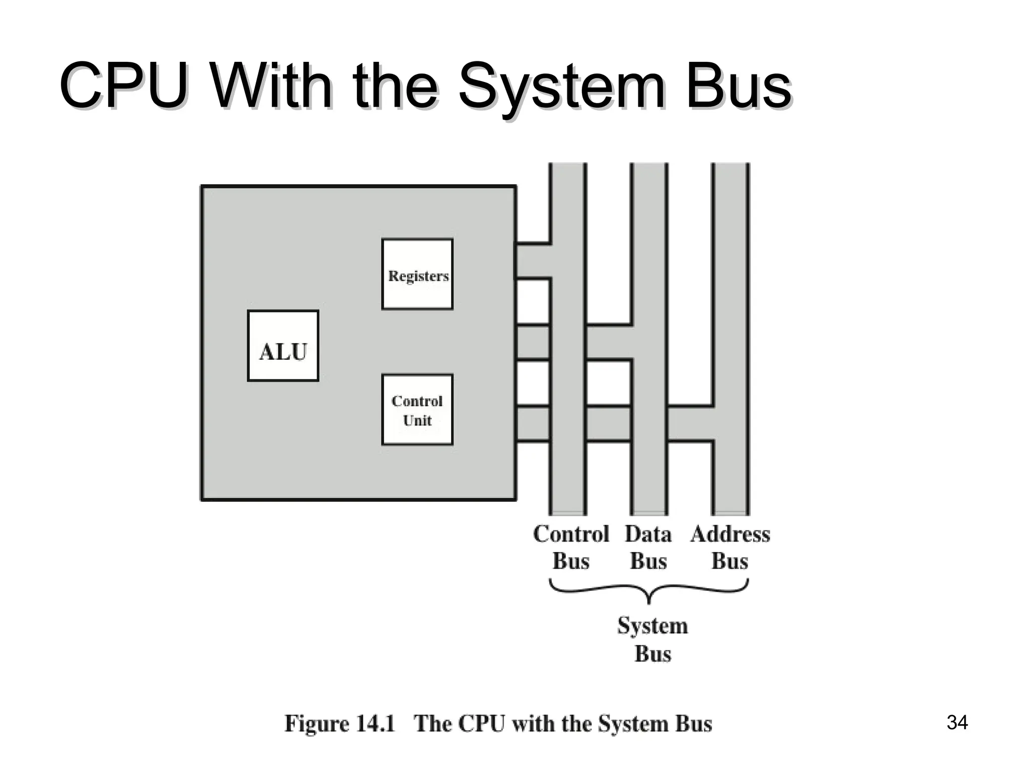
#34 Figure 14.1 is a simplified view of a processor, indicating its connection to the rest of the system via the system bus. A similar interface would be needed for any of the interconnection structures described in Chapter 3. The reader will recall that the major components of the processor are an arithmetic and logic unit (ALU) and a control unit (CU). The ALU does the actual computation or processing of data. The control unit controls the movement of data and instructions into and out of the processor and controls the operation of the ALU. In addition, the figure shows a minimal internal memory, consisting of a set of storage locations, called registers.
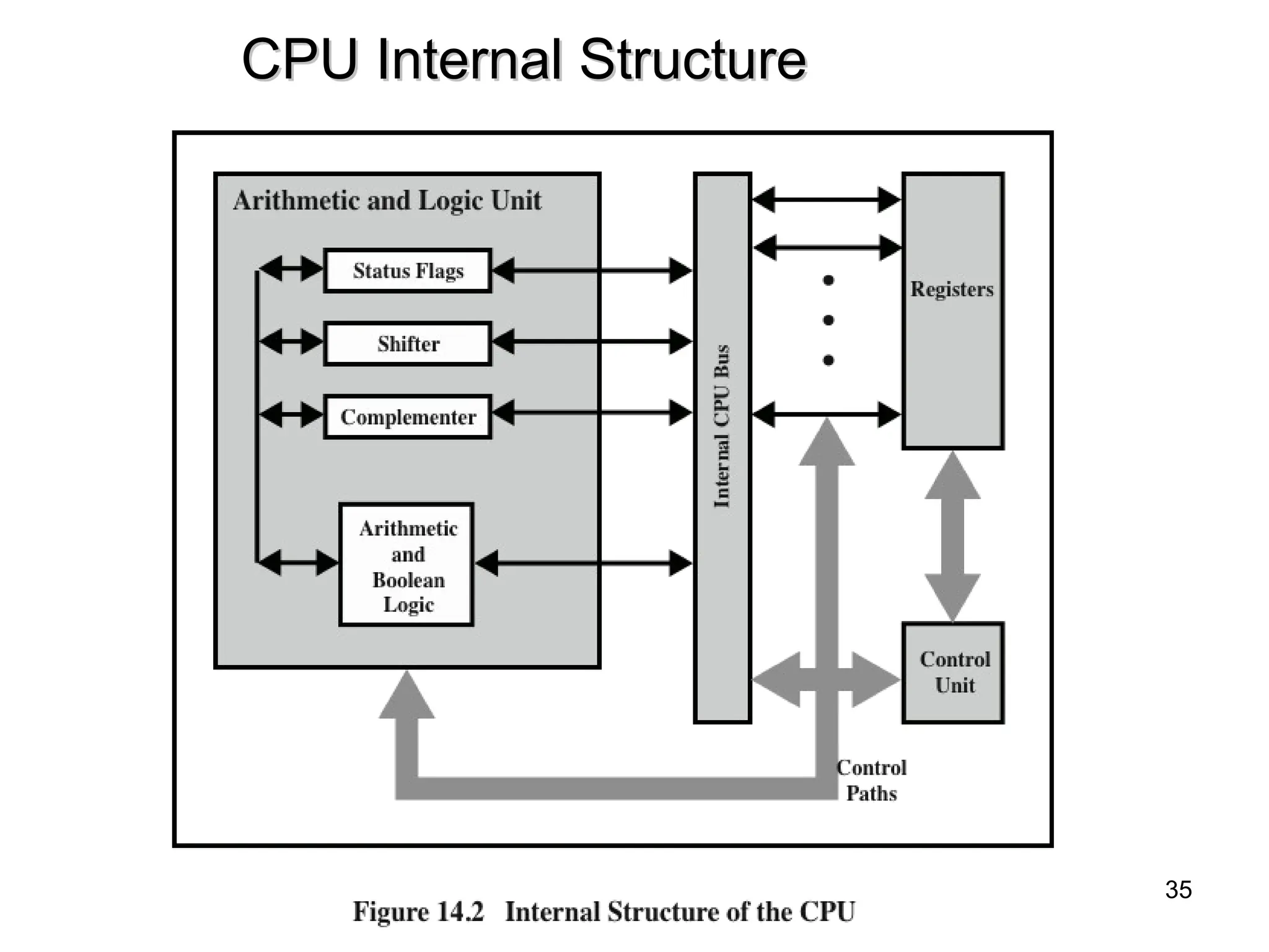
#35 Figure 14.2 is a slightly more detailed view of the processor. The data transfer and logic control paths are indicated, including an element labeled internal
processor bus. This element is needed to transfer data between the various registers and the ALU because the ALU in fact operates only on data in the internal processor memory. The figure also shows typical basic elements of the ALU. Note the similarity between the internal structure of the computer as a whole and the internal structure of the processor. In both cases, there is a small collection of major elements (computer: processor, I/O, memory; processor: control unit, ALU, registers) connected by data paths.
#36 As we discussed in Chapter 4, a computer system employs a memory hierarchy. At higher levels of the hierarchy, memory is faster, smaller, and more expensive (per bit). Within the processor, there is a set of registers that function as a level of memory above main memory and cache in the hierarchy. The registers in the processor perform two roles:
User-visible registers: Enable the machine- or assembly language programmer to minimize main memory references by optimizing use of registers.
Control and status registers: Used by the control unit to control the operation of the processor and by privileged, operating system programs to control the execution of programs.
There is not a clean separation of registers into these two categories. For example, on some machines the program counter is user visible (e.g., x86), but on many it is not. For purposes of the following discussion, however, we will use these categories.
#38 There are a variety of processor registers that are employed to control the operation of the processor. Most of these, on most machines, are not visible to the user. Some of them may be visible to machine instructions executed in a control or operating system mode.
Of course, different machines will have different register organizations and use different terminology. We list here a reasonably complete list of register types, with a brief description.
Four registers are essential to instruction execution:
Program counter (PC): Contains the address of an instruction to be fetched.
Instruction register (IR): Contains the instruction most recently fetched.
Memory address register (MAR): Contains the address of a location in memory.
Memory buffer register (MBR): Contains a word of data to be written to memory or the word most recently read.
Not all processors have internal registers designated as MAR and MBR, but some equivalent buffering mechanism is needed whereby the bits to be transferred to the system bus are staged and the bits to be read from the data bus are temporarily stored.
Typically, the processor updates the PC after each instruction fetch so that the PC always points to the next instruction to be executed. A branch or skip instruction will also modify the contents of the PC. The fetched instruction is loaded into an IR, where the opcode and operand specifiers are analyzed. Data are exchanged with memory using the MAR and MBR. In a bus- organized system, the MAR connects directly to the address bus, and the MBR connects directly to the data bus. User-visible registers, in turn, exchange data with the MBR.
The four registers just mentioned are used for the movement of data between the processor and memory. Within the processor, data must be presented to the ALU for processing. The ALU may have direct access to the MBR and user-visible registers. Alternatively, there may be additional buffering registers at the boundary to the ALU; these registers serve as input and output registers for the ALU and exchange data with the MBR and user-visible registers.
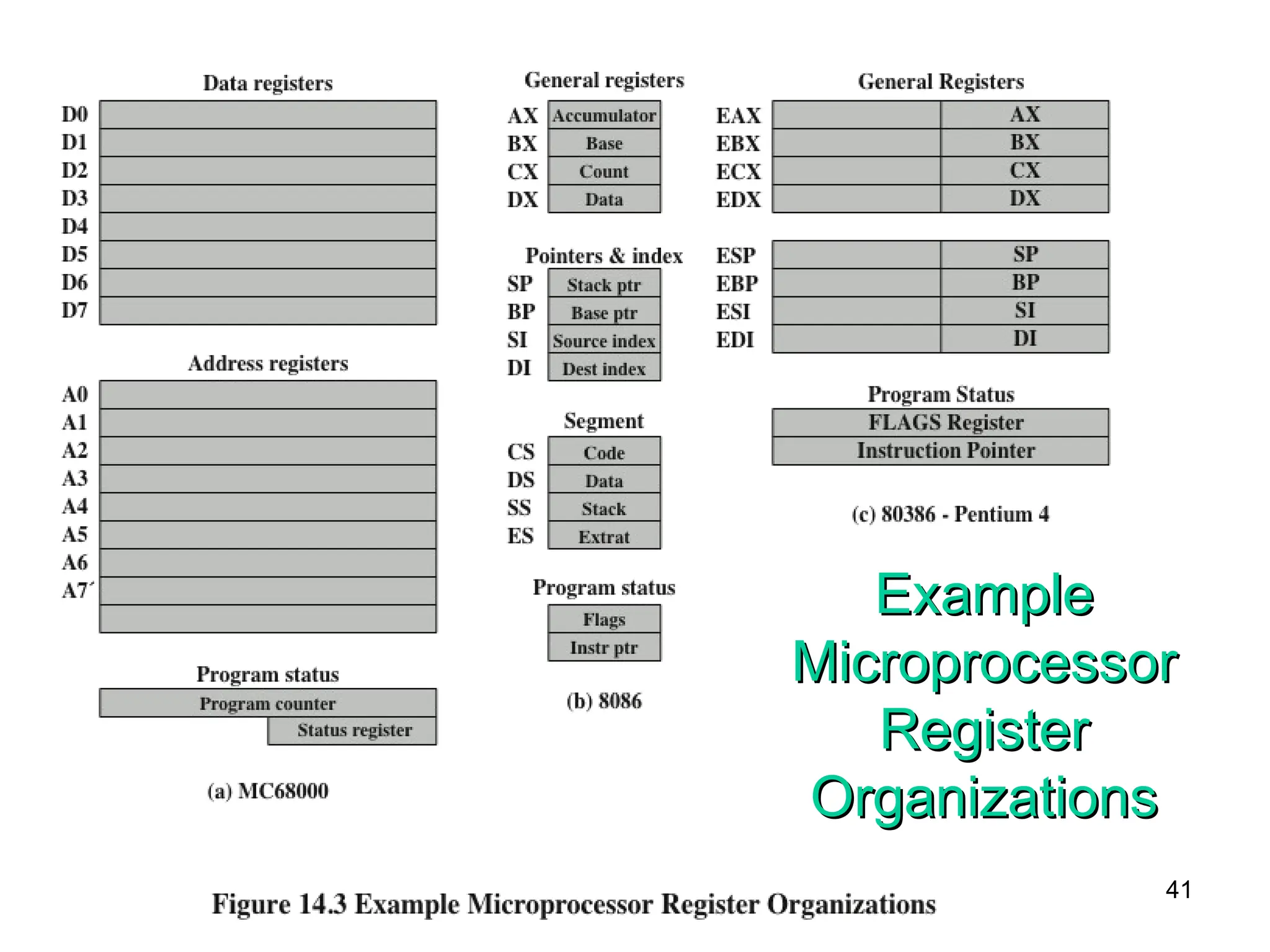
#41 It is instructive to examine and compare the register organization of comparable systems. In this section, we look at two 16-bit microprocessors that were designed at about the same time: the Motorola MC68000 [STRI79] and the Intel 8086 [MORS78]. Figures 14.3a and b depict the register organization of each; purely internal registers, such as a memory address register, are not shown.
The MC68000 partitions its 32-bit registers into eight data registers and nine address registers. The eight data registers are used primarily for data manipulation and are also used in addressing as index registers. The width of the registers allows 8-, 16-, and 32-bit data operations, determined by opcode. The address registers contain 32-bit (no segmentation) addresses; two of these registers are also used as stack pointers, one for users and one for the operating system, depending on the current execution mode. Both registers are numbered 7, because only one can be used at a time. The MC68000 also includes a 32-bit program counter and a 16-bit status register.
The Intel 8086 takes a different approach to register organization. Every register is special purpose, although some registers are also usable as general purpose. The 8086 contains four 16-bit data registers that are addressable on a byte or 16-bit basis, and four 16-bit pointer and index registers. The data registers can be used as general purpose in some instructions. In others, the registers are used implicitly. For example, a multiply instruction always uses the accumulator. The four pointer registers are also used implicitly in a number of operations; each contains a segment offset. There are also four 16-bit segment registers. Three of the four segment registers are used in a dedicated, implicit fashion, to point to the segment of the current instruction (useful for branch instructions), a segment containing data, and a segment containing a stack, respectively. These dedicated and implicit uses provide for compact encoding at the cost of reduced flexibility. The 8086 also includes an instruction pointer and a set of 1-bit status and control flags.
The point of this comparison should be clear. There is no universally accepted philosophy concerning the best way to organize processor registers [TOON81]. As with overall instruction set design and so many other processor design issues, it is still a matter of judgment and taste.
A second instructive point concerning register organization design is illustrated in Figure 14.3c. This figure shows the user-visible register organization for the Intel 80386 [ELAY85], which is a 32-bit microprocessor designed as an extension of the 8086.1 The 80386 uses 32-bit registers. However, to provide upward compatibility for programs written on the earlier machine, the 80386 retains the original register organization embedded in the new organization. Given this design constraint, the architects of the 32-bit processors had limited flexibility in designing the register organization.

![Number of Addresses
• More addresses
– More complex (powerful?) instructions
– More registers - inter-register operations are quicker
– Less instructions per program
• Fewer addresses
– Less complex (powerful?) instructions
– More instructions per program, e.g. data movement
– Faster fetch/execution of instructions
• Example: Y=(A-B):[(C+(DxE)]
11](https://image.slidesharecdn.com/ch3thecpumodified-250304074729-de43a758/75/ch-3_The-CPU_modified-ppt-of-central-processing-unit-11-2048.jpg)