Variability, the normal distribution and converted scoresNema Grace Medillo
Understanding mean and standard deviation in the normal distribution curve, Understanding scores using range, semi-interquartile range, standard deviation and variance. Converting scores through z- scores and t - scores,
Variability, the normal distribution and converted scoresNema Grace Medillo
Understanding mean and standard deviation in the normal distribution curve, Understanding scores using range, semi-interquartile range, standard deviation and variance. Converting scores through z- scores and t - scores,
Explore our comprehensive data analysis project presentation on predicting product ad campaign performance. Learn how data-driven insights can optimize your marketing strategies and enhance campaign effectiveness. Perfect for professionals and students looking to understand the power of data analysis in advertising. for more details visit: https://bostoninstituteofanalytics.org/data-science-and-artificial-intelligence/
Adjusting primitives for graph : SHORT REPORT / NOTESSubhajit Sahu
Graph algorithms, like PageRank Compressed Sparse Row (CSR) is an adjacency-list based graph representation that is
Multiply with different modes (map)
1. Performance of sequential execution based vs OpenMP based vector multiply.
2. Comparing various launch configs for CUDA based vector multiply.
Sum with different storage types (reduce)
1. Performance of vector element sum using float vs bfloat16 as the storage type.
Sum with different modes (reduce)
1. Performance of sequential execution based vs OpenMP based vector element sum.
2. Performance of memcpy vs in-place based CUDA based vector element sum.
3. Comparing various launch configs for CUDA based vector element sum (memcpy).
4. Comparing various launch configs for CUDA based vector element sum (in-place).
Sum with in-place strategies of CUDA mode (reduce)
1. Comparing various launch configs for CUDA based vector element sum (in-place).
Levelwise PageRank with Loop-Based Dead End Handling Strategy : SHORT REPORT ...Subhajit Sahu
Abstract — Levelwise PageRank is an alternative method of PageRank computation which decomposes the input graph into a directed acyclic block-graph of strongly connected components, and processes them in topological order, one level at a time. This enables calculation for ranks in a distributed fashion without per-iteration communication, unlike the standard method where all vertices are processed in each iteration. It however comes with a precondition of the absence of dead ends in the input graph. Here, the native non-distributed performance of Levelwise PageRank was compared against Monolithic PageRank on a CPU as well as a GPU. To ensure a fair comparison, Monolithic PageRank was also performed on a graph where vertices were split by components. Results indicate that Levelwise PageRank is about as fast as Monolithic PageRank on the CPU, but quite a bit slower on the GPU. Slowdown on the GPU is likely caused by a large submission of small workloads, and expected to be non-issue when the computation is performed on massive graphs.
Show drafts
volume_up
Empowering the Data Analytics Ecosystem: A Laser Focus on Value
The data analytics ecosystem thrives when every component functions at its peak, unlocking the true potential of data. Here's a laser focus on key areas for an empowered ecosystem:
1. Democratize Access, Not Data:
Granular Access Controls: Provide users with self-service tools tailored to their specific needs, preventing data overload and misuse.
Data Catalogs: Implement robust data catalogs for easy discovery and understanding of available data sources.
2. Foster Collaboration with Clear Roles:
Data Mesh Architecture: Break down data silos by creating a distributed data ownership model with clear ownership and responsibilities.
Collaborative Workspaces: Utilize interactive platforms where data scientists, analysts, and domain experts can work seamlessly together.
3. Leverage Advanced Analytics Strategically:
AI-powered Automation: Automate repetitive tasks like data cleaning and feature engineering, freeing up data talent for higher-level analysis.
Right-Tool Selection: Strategically choose the most effective advanced analytics techniques (e.g., AI, ML) based on specific business problems.
4. Prioritize Data Quality with Automation:
Automated Data Validation: Implement automated data quality checks to identify and rectify errors at the source, minimizing downstream issues.
Data Lineage Tracking: Track the flow of data throughout the ecosystem, ensuring transparency and facilitating root cause analysis for errors.
5. Cultivate a Data-Driven Mindset:
Metrics-Driven Performance Management: Align KPIs and performance metrics with data-driven insights to ensure actionable decision making.
Data Storytelling Workshops: Equip stakeholders with the skills to translate complex data findings into compelling narratives that drive action.
Benefits of a Precise Ecosystem:
Sharpened Focus: Precise access and clear roles ensure everyone works with the most relevant data, maximizing efficiency.
Actionable Insights: Strategic analytics and automated quality checks lead to more reliable and actionable data insights.
Continuous Improvement: Data-driven performance management fosters a culture of learning and continuous improvement.
Sustainable Growth: Empowered by data, organizations can make informed decisions to drive sustainable growth and innovation.
By focusing on these precise actions, organizations can create an empowered data analytics ecosystem that delivers real value by driving data-driven decisions and maximizing the return on their data investment.
1. 10
Z-score
(Standardized Normal Deviate)
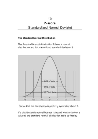
The Standard Normal Distribution
The Standard Normal distribution follows a normal
distribution and has mean 0 and standard deviation 1
Notice that the distribution is perfectly symmetric about 0.
If a distribution is normal but not standard, we can convert a
value to the Standard normal distribution table by first by
2. Biostatistics-77
finding how many standard deviations away the number is
from the mean.
The z-score
[Q: Write short notes on: Z-score. (BSMMU, MD Radiology,
July, 2010)]
The number of standard deviations from the mean is called
the z-score and can be found by the formula
x
z
Explanation:
How would you compare the number of books in ‘library A’
to the number of books in other libraries? What type of
statistic would you use to actually give information about
‘library A’, short of counting every book in several different
libraries?
You would use a standard score. Standard scores are
calculated in order to describe the extent of variation of a
value as it would be compared to another value. They are the
most convenient way to compare similar or different values
by a similar scale.
If ‘library A’ contains 250 books, you won’t be able to tell how
that number compares to other libraries, such as that of the
average college professor. To more effectively describe
‘library A’ in comparison to other libraries, we calculate a
standard score or z-score. The standard score number
3. Biostatistics-78
describes the location of a particular case in a distribution:
whether it is above or below the average and by how much.
The z-score is expressed in standard deviation units, so it
always gives you an idea of the magnitude of the difference
compared to the distribution of values for the whole
population.
To calculate the z-score of a value x from a distribution one
needs the mean and the standard deviation for that
distribution. The formula reads:
x
z
In the library example, if book ownership among college
professors has a mean of 150 and a standard deviation of
50, the z-score for library A (consisting of 250 books) is:
2
50
150
250
z
The z-score for library A is positive, indicating it has more
books than average. It tells us that library A is two standard
deviations over the mean. Now you probably will remember
the empirical rule for bell-shaped distribution, which tells us
that
approximately 68% of all observations is less than 1
standard deviation away from the mean, and
approximately 95% of all observations is less than 2
standard deviations away from the mean,
so we now have a pretty good idea about the magnitude of
library A compared to other ones. This particular library is
5. Biostatistics-80
To conclude: z-scores inform us in a standardized way about
the position of an observation within a certain distribution.
Example
Find the z-score corresponding to a raw score of 132 from a
normal distribution with mean 100 and standard deviation 15.
Solution
We compute
132 - μ
z = = 2.133
15
Example
A z-score of 1.7 was found from an observation coming from
a normal distribution with mean 14 and standard deviation 3.
Find the raw score.
Solution
We have
x - μ
1.7 =
3
To solve this we just multiply both sides by the denominator
3,
6. Biostatistics-81
(1.7)(3) = x - 14
5.1 = x - 14
x = 19.1
The z-score and Area
Often we want to find the probability that a z-score will be
less than a given value, greater than a given value, or in
between two values. To accomplish this, we use the table
from the textbook and a few properties about the normal
distribution.
Example
Find
P(z < 2.37)
7. Biostatistics-82
Solution
We use the table. Notice the picture on the table has shaded
region corresponding to the area to the left (below) a z-
score. This is exactly what we want. Below are a few lines of
the table.
z .00 .01 .02 .03 .04 .05 .06 .07 .08 .09
2.2 .9861 .9864 .9868 .9871 .9875 .9878 .9881 .9884 .9887 .9890
2.3 .9893 .9896 .9898 .9901 .9904 .9906 .9909 .9911 .9913 .9916
2.4 .9918 .9920 .9922 .9925 .9927 .9929 .9931 .9932 .9934 .9936
The columns corresponds to the ones and tenths digits of the
z-score and the rows correspond to the hundredths digits.
For our problem we want the row 2.3 (from 2.37) and the row
.07 (from 2.37). The number in the table that matches this is
.9911.
Hence
P(z < 2.37) = .9911
Example
Find
P(z > 1.82)
Solution
8. Biostatistics-83
In this case, we want the area to the right of 1.82. This is not
what is given in the table. We can use the identity
P(z > 1.82) = 1 - P(z < 1.82)
reading the table gives
P(z < 1.82) = .9656
Our answer is
P(z > 1.82) = 1 - .9656 = .0344
Example
Find P(-1.18 < z < 2.1)
Solution
9. Biostatistics-84
Once again, the table does not exactly handle this type of
area. However, the area between -1.18 and 2.1 is equal to the
area to the left of 2.1 minus the area to the left of -1.18. That
is
P(-1.18 < z < 2.1) = P(z < 2.1) - P(z < -1.18)
To find P(z < 2.1) we rewrite it as P(z < 2.10) and use the table
to get
P(z < 2.10) = .9821.
The table also tells us that
P(z < -1.18) = .1190
Now subtract to get
P(-1.18 < z < 2.1) = .9821 - .1190 = .8631
![Biostatistics-77
finding how many standard deviations away the number is
from the mean.
The z-score
[Q: Write short notes on: Z-score. (BSMMU, MD Radiology,
July, 2010)]
The number of standard deviations from the mean is called
the z-score and can be found by the formula
x
z
Explanation:
How would you compare the number of books in ‘library A’
to the number of books in other libraries? What type of
statistic would you use to actually give information about
‘library A’, short of counting every book in several different
libraries?
You would use a standard score. Standard scores are
calculated in order to describe the extent of variation of a
value as it would be compared to another value. They are the
most convenient way to compare similar or different values
by a similar scale.
If ‘library A’ contains 250 books, you won’t be able to tell how
that number compares to other libraries, such as that of the
average college professor. To more effectively describe
‘library A’ in comparison to other libraries, we calculate a
standard score or z-score. The standard score number](data:image/gif;base64,R0lGODlhAQABAIAAAAAAAP///yH5BAEAAAAALAAAAAABAAEAAAIBRAA7)