The ROC curve is a graph that plots the true positive rate against the false positive rate for different cut-points of a diagnostic test. It shows the relationship between sensitivity and specificity as the cut-point is varied. Moving the cut-point to require a higher test result for a positive diagnosis improves sensitivity but reduces specificity, and vice versa. The closer the ROC curve follows the top left corner, the more accurate the test. The area under the curve provides a measure of test accuracy. The ROC curve was originally developed in WWII for analyzing radar images but is now widely used for evaluating medical diagnostic tests.

1. 18
ROC Curve
(Receiver Operating Characteristic curve)
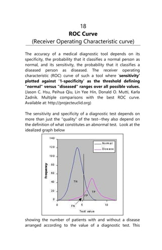
The accuracy of a medical diagnostic tool depends on its
specificity, the probability that it classifies a normal person as
normal, and its sensitivity, the probability that it classifies a
diseased person as diseased. The receiver operating
characteristic (ROC) curve of such a tool where ‘sensitivity’
plotted against ‘1-specificity’ as the threshold defining
"normal" versus "diseased" ranges over all possible values.
(Jason C. Hsu, Peihua Qiu, Lin Yee Hin, Donald O. Mutti, Karla
Zadnik. Multiple comparisons with the best ROC curve.
Available at: http://projecteuclid.org)
The sensitivity and specificity of a diagnostic test depends on
more than just the "quality" of the test--they also depend on
the definition of what constitutes an abnormal test. Look at the
idealized graph below
showing the number of patients with and without a disease
arranged according to the value of a diagnostic test. This

2. Biostatistics-153
distributions overlap--the test (like most) does not distinguish
normal from disease with 100% accuracy.
The area of overlap indicates where the test cannot distinguish
normal from disease. In practice, we choose a cutpoint
(indicated by the vertical black line) above which we consider
the test to be abnormal and below which we consider the test
to be normal. The position of the cutpoint will determine the
number of true positive, true negatives, false positives and false
negatives. We may wish to use different cutpoints for different
clinical situations if we wish to minimize one of the erroneous
types of test results.
Example: Patients with Suspected Hypothyroidism
Consider the following data on patients with suspected
hypothyroidism reported by Goldstein and Mushlin (J Gen
Intern Med 1987;2:20-24.). They measured T4 and TSH values in
ambulatory patients with suspected hypothyroidism and used
the TSH values as a gold standard for determining which
patients were truly hypothyroid.
T4 value Hypothyroid Euthyroid
5 or less 18 1
5.1 - 7 7 17
7.1 - 9 4 36
9 or more 3 39
Totals: 32 93
Notice that these authors found considerable overlap in T4
values among the hypothyroid and euthyroid patients
 Suppose that patients with T4 values of 5 or less are
considered to be hypothyroid. The data display then
reduces to:

3. Biostatistics-154
T4 value Hypothyroid Euthyroid
5 or less 18 1
> 5 14 92
Totals: 32 93
You should be able to verify that the sensivity is 0.56 and the
specificity is 0.99.
 Now, suppose we decide to make the definition of
hypothyroidism less stringent and now consider patients
with T4 values of 7 or less to be hypothyroid. The data
display will now look like this:
T4 value Hypothyroid Euthyroid
7 or less 25 18
> 7 7 75
Totals: 32 93
You should be able to verify that the sensivity is 0.78 and the
specificity is 0.81.
 Lets move the cut point for hypothyroidism one more time:
T4 value Hypothyroid Euthyroid
< 9 29 54
9 or more 3 39
Totals: 32 93
You should be able to verify that the sensivity is 0.91 and the
specificity is 0.42.
Now, take the sensitivity and specificity values above and put
them into a table:
Cutpoint Sensitivity Specificity
5 0.56 0.99
7 0.78 0.81
9 0.91 0.42

4. Biostatistics-155
Notice that you can improve the sensitivity by moving to
cutpoint to a higher T4 value--that is, you can make the
criterion for a positive test less strict. You can improve the
specificity by moving the cutpoint to a lower T4 value--that is,
you can make the criterion for a positive test more strict. Thus,
there is a transaction between sensitivity and specificity. You
can change the definition of a positive test to improve one but
the other will decline.
Plotting and Intrepretating an ROC Curve
The operating characteristics (above table) can be reformulated
slightly as follows
Cutpoint True positive rates
(Sensitivity)
False positive rates
(1-Specificity)
5 0.56 0.01
7 0.78 0.19
9 0.91 0.58
Data of the above table can be plotted graphically as shown
below

5. Biostatistics-156
This type of graph is called a Receiver Operating
Characteristic curve (or ROC curve.) It is a plot of the true
positive rate against the false positive rate for the different
possible cutpoints of a diagnostic test.
An ROC curve demonstrates several things:
1. It shows the transaction between sensitivity and
specificity (any increase in sensitivity will be
accompanied by a decrease in specificity).
2. The closer the curve follows the left-hand border and
then the top border of the ROC space, the more
accurate the test.
3. The closer the curve comes to the 45-degree diagonal
of the ROC space, the less accurate the test.
4. The area under the curve is a measure of text accuracy.
A final note of historical interest

6. Biostatistics-157
You may be wondering where the name "Reciever Operating
Characteristic" came from. ROC analysis is part of a field called
"Signal Dectection Therory" developed during World War II for
the analysis of radar images. Radar operators had to decide
whether a blip on the screen represented an enemy target, a
friendly ship, or just noise. Signal detection theory measures
the ability of radar receiver operators to make these important
distinctions. Their ability to do so was called the Receiver
Operating Characteristics. It was not until the 1970's that signal
detection theory was recognized as useful for interpreting
medical test results.
[Q: write short note on: ROC curve. (BSMMU, MD Radiology,
January, 2009)]