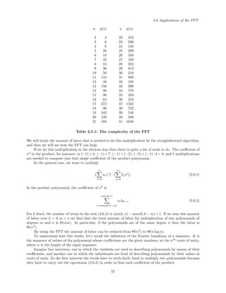
The document is a text by Herbert S. Wilf about algorithms and complexity, covering various topics related to solving computational problems effectively and analyzing their efficiency, particularly in terms of time and space complexity. It includes chapters on mathematical preliminaries, recursive algorithms, network flow problems, algorithms in number theory, and NP-completeness, aimed at computer science and mathematics students. The content is structured to provide foundational knowledge and practical programming exercises to enhance learning outcomes in algorithms.

![1.5 Counting
8. Write out a complete proof of theorem 1.4.1.
9. Show by an example that the conclusion of theorem 1.4.1 may be false if the phrase ‘for every fixed
> 0 . . .’ were replaced by ‘for every fixed ≥ 0 . . ..’
10. In theorem 1.4.1 we find the phrase ‘... the positive real root of ...’ Prove that this phrase is justified, in
that the equation shown always has exactly one positive real root. Exactly what special properties of that
equation did you use in your proof?
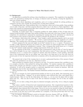
1.5 Counting
For a given positive integer n, consider the set {1, 2, . . .n}. We will denote this set by the symbol [n],
and we want to discuss the number of subsets of various kinds that it has. Here is a list of all of the subsets
of [2]: ∅, {1}, {2}, {1, 2}. There are 4 of them.
We claim that the set [n] has exactly 2n
subsets.
To see why, notice that we can construct the subsets of [n] in the following way. Either choose, or don’t
choose, the element ‘1,’ then either choose, or don’t choose, the element ‘2,’ etc., finally choosing, or not
choosing, the element ‘n.’ Each of the n choices that you encountered could have been made in either of 2
ways. The totality of n choices, therefore, might have been made in 2n
different ways, so that is the number
of subsets that a set of n objects has.
Next, suppose we have n distinct objects, and we want to arrange them in a sequence. In how many
ways can we do that? For the first object in our sequence we may choose any one of the n objects. The
second element of the sequence can be any of the remaining n − 1 objects, so there are n(n − 1) possible
ways to make the first two decisions. Then there are n − 2 choices for the third element, and so we have
n(n − 1)(n − 2) ways to arrange the first three elements of the sequence. It is no doubt clear now that there
are exactly n(n − 1)(n − 2) · · · 3 · 2 · 1 = n! ways to form the whole sequence.
Of the 2n
subsets of [n], how many have exactly k objects in them? The number of elements in a
set is called its cardinality. The cardinality of a set S is denoted by |S|, so, for example, |[6]| = 6. A set
whose cardinality is k is called a ‘k-set,’ and a subset of cardinality k is, naturally enough, a ‘k-subset.’ The
question is, for how many subsets S of [n] is it true that |S| = k?
We can construct k-subsets S of [n] (written ‘S ⊆ [n]’) as follows. Choose an element a1 (n possible
choices). Of the remaining n − 1 elements, choose one (n − 1 possible choices), etc., until a sequence of k
different elements have been chosen. Obviously there were n(n − 1)(n − 2) · · · (n − k + 1) ways in which we
might have chosen that sequence, so the number of ways to choose an (ordered) sequence of k elements from
[n] is
n(n − 1)(n − 2) · · · (n − k + 1) = n!/(n − k)!.
But there are more sequences of k elements than there are k-subsets, because any particular k-subset S
will correspond to k! different ordered sequences, namely all possible rearrangements of the elements of the
subset. Hence the number of k-subsets of [n] is equal to the number of k-sequences divided by k!. In other
words, there are exactly n!/k!(n − k)! k-subsets of a set of n objects.
The quantities n!/k!(n − k)! are the famous binomial coefficients, and they are denoted by
n
k
=
n!
k!(n − k)!
(n ≥ 0; 0 ≤ k ≤ n). (1.5.1)
Some of their special values are
n
0
= 1 (∀n ≥ 0);
n
1
= n (∀n ≥ 0);
n
2
= n(n − 1)/2 (∀n ≥ 0);
n
n
= 1 (∀n ≥ 0).
It is convenient to define n
k to be 0 if k < 0 or if k > n.
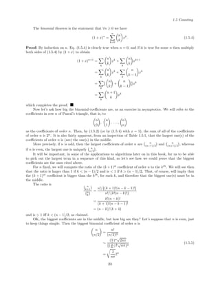
We can summarize the developments so far with
21](https://image.slidesharecdn.com/algorithmsandcomplexity-160122031826/85/Algorithms-andcomplexity-25-320.jpg)
![Chapter 1: Mathematical Preliminaries
Theorem 1.5.1. For each n ≥ 0, a set of n objects has exactly 2n
subsets, and of these, exactly n
k have
cardinality k ( ∀k = 0, 1, . . . , n). There are exactly n! different sequences that can be formed from a set of n
distinct objects.
Since every subset of [n] has some cardinality, it follows that
n
k=0
n
k
= 2n
(n = 0, 1, 2, . . .). (1.5.2)
In view of the convention that we adopted, we might have written (1.5.2) as k
n
k = 2n
, with no restriction
on the range of the summation index k. It would then have been understood that the range of k is from
−∞ to ∞, and that the binomial coefficient n
k vanishes unless 0 ≤ k ≤ n.
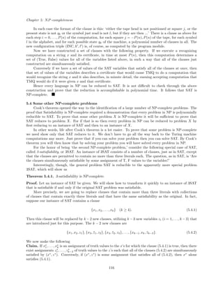
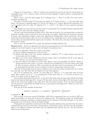
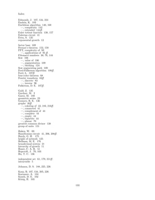
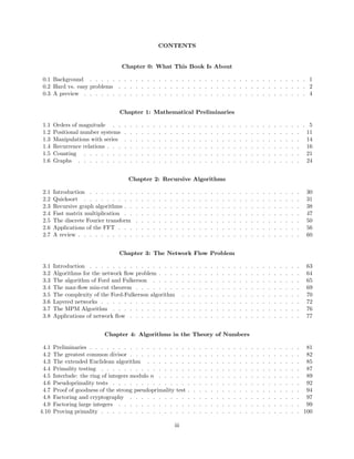
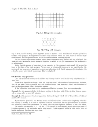
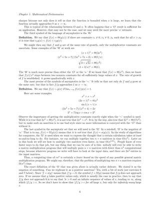
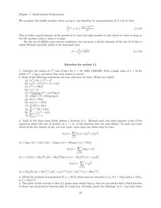
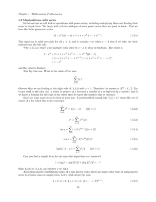
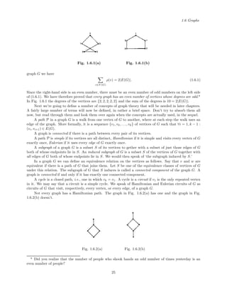
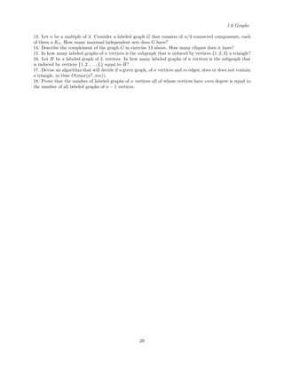
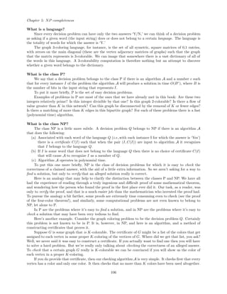
In Table 1.5.1 we show the values of some of the binomial coefficients n
k . The rows of the table
are thought of as labelled ‘n = 0,’ ‘n = 1,’ etc., and the entries within each row refer, successively, to
k = 0, 1, . . ., n. The table is called ‘Pascal’s triangle.’
1
1 1
1 2 1
1 3 3 1
1 4 6 4 1
1 5 10 10 5 1
1 6 15 20 15 6 1
1 7 21 35 35 21 7 1
1 8 28 56 70 56 28 8 1
...................................................
..
Table 1.5.1: Pascal’s triangle
Here are some facts about the binomial coefficients:
(a) Each row of Pascal’s triangle is symmetric about the middle. That is,
n
k
=
n
n − k
(0 ≤ k ≤ n; n ≥ 0).
(b) The sum of the entries in the nth
row of Pascal’s triangle is 2n
.
(c) Each entry is equal to the sum of the two entries that are immediately above it in the triangle.
The proof of (c) above can be interesting. What it says about the binomial coefficients is that
n
k
=
n − 1
k − 1
+
n − 1
k
((n, k) = (0, 0)). (1.5.3)
There are (at least) two ways to prove (1.5.3). The hammer-and-tongs approach would consist of expanding
each of the three binomial coefficients that appears in (1.5.3), using the definition (1.5.1) in terms of factorials,
and then cancelling common factors to complete the proof.
That would work (try it), but here’s another way. Contemplate (this proof is by contemplation) the
totality of k-subsets of [n]. The number of them is on the left side of (1.5.3). Sort them out into two piles:
those k-subsets that contain ‘1’ and those that don’t. If a k-subset of [n] contains ‘1,’ then its remaining
k − 1 elements can be chosen in n−1
k−1 ways, and that accounts for the first term on the right of (1.5.3). If a
k-subset does not contain ‘1,’ then its k elements are all chosen from [n − 1], and that completes the proof
of (1.5.3).
22](https://image.slidesharecdn.com/algorithmsandcomplexity-160122031826/85/Algorithms-andcomplexity-26-320.jpg)
![Chapter 1: Mathematical Preliminaries
where we have used Stirling’s formula (1.1.10).
Equation (1.5.5) shows that the single biggest binomial coefficient accounts for a very healthy fraction
of the sum of all of the coefficients of order n. Indeed, the sum of all of them is 2n
, and the biggest one is
∼ 2/nπ2n
. When n is large, therefore, the largest coefficient contributes a fraction ∼ 2/nπ of the total.
If we think in terms of the subsets that these coefficients count, what we will see is that a large fraction
of all of the subsets of an n-set have cardinality n/2, in fact Θ(n−.5
) of them do. This kind of probabilistic
thinking can be very useful in the design and analysis of algorithms. If we are designing an algorithm that
deals with subsets of [n], for instance, we should recognize that a large percentage of the customers for that
algorithm will have cardinalities near n/2, and make every effort to see that the algorithm is fast for such
subsets, even at the expense of possibly slowing it down on subsets whose cardinalities are very small or very
large.
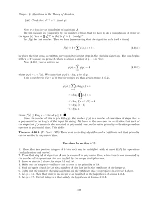
Exercises for section 1.5
1. How many subsets of even cardinality does [n] have?
2. By observing that (1 + x)a
(1 + x)b
= (1 + x)a+b
, prove that the sum of the squares of all binomial
coefficients of order n is 2n
n .
3. Evaluate the following sums in simple form.
(i)
n
j=0 j n
j
(ii)
n
j=3
n
j 5j
(iii)
n
j=0(j + 1)3j+1
4. Find, by direct application of Taylor’s theorem, the power series expansion of f(x) = 1/(1 − x)m+1
about
the origin. Express the coefficients as certain binomial coefficients.
5. Complete the following twiddles.
(i) 2n
n ∼ ?
(ii) n
log2 n ∼ ?
(iii) n
θn ∼ ?
(iv) n2
n ∼ ?
6. How many ordered pairs of unequal elements of [n] are there?
7. Which one of the numbers {2j n
j }n
j=0 is the biggest?
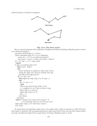
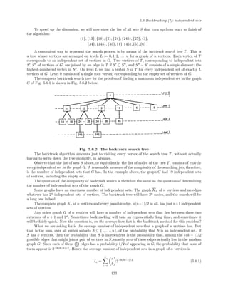
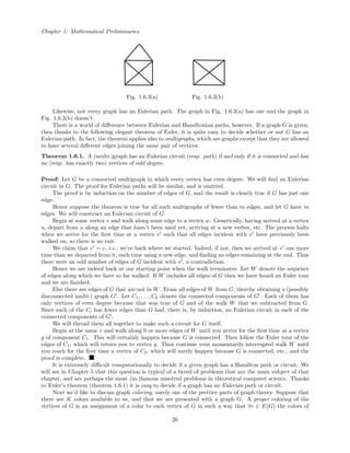
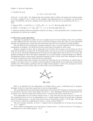
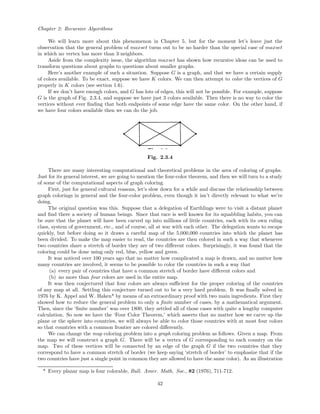
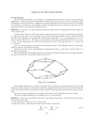
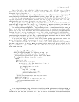
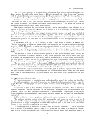
1.6 Graphs
A graph is a collection of vertices, certain unordered pairs of which are called its edges. To describe a
particular graph we first say what its vertices are, and then we say which pairs of vertices are its edges. The
set of vertices of a graph G is denoted by V (G), and its set of edges is E(G).
If v and w are vertices of a graph G, and if (v, w) is an edge of G, then we say that vertices v, w are
adjacent in G.
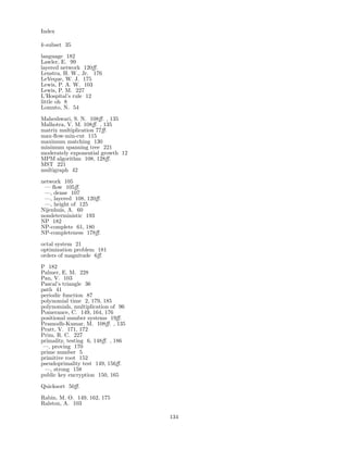
Consider the graph G whose vertex set is {1, 2, 3, 4, 5} and whose edges are the set of pairs (1,2), (2,3),
(3,4), (4,5), (1,5). This is a graph of 5 vertices and 5 edges. A nice way to present a graph to an audience
is to draw a picture of it, instead of just listing the pairs of vertices that are its edges. To draw a picture of
a graph we would first make a point for each vertex, and then we would draw an arc between two vertices v
and w if and only if (v, w) is an edge of the graph that we are talking about. The graph G of 5 vertices and
5 edges that we listed above can be drawn as shown in Fig. 1.6.1(a). It could also be drawn as shown in
Fig. 1.6.1(b). They’re both the same graph. Only the pictures are different, but the pictures aren’t ‘really’
the graph; the graph is the vertex list and the edge list. The pictures are helpful to us in visualizing and
remembering the graph, but that’s all.
The number of edges that contain (‘are incident with’) a particular vertex v of a graph G is called the
degree of that vertex, and is usually denoted by ρ(v). If we add up the degrees of every vertex v of G we will
have counted exactly two contributions from each edge of G, one at each of its endpoints. Hence, for every
24](https://image.slidesharecdn.com/algorithmsandcomplexity-160122031826/85/Algorithms-andcomplexity-28-320.jpg)
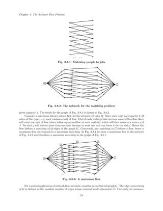
![2.2 Quicksort
procedure calculate(list of variables);
if {trivialcase} then do {trivialthing}
else do
{call calculate(smaller values of the variables)};
{maybe do a few more things}
end.
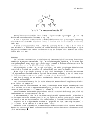
In this chapter we’re going to work out a number of examples of recursive algorithms, of varying
sophistication. We will see how the recursive structure helps us to analyze the running time, or complexity,
of the algorithms. We will also find that there is a bit of art involved in choosing the list of variables that
a recursive procedure operates on. Sometimes the first list we think of doesn’t work because the recursive
call seems to need more detailed information than we have provided for it. So we try a larger list, and then
perhaps it works, or maybe we need a still larger list ..., but more of this later.
Exercises for section 2.1
1. Write a recursive routine that will find the digits of a given integer n in the base b. There should be no
visible loops in your program.
2.2 Quicksort
Suppose that we are given an array x[1], . . . , x[n] of n numbers. We would like to rearrange these
numbers as necessary so that they end up in nondecreasing order of size. This operation is called sorting the
numbers.
For instance, if we are given {9, 4, 7, 2, 1}, then we want our program to output the sorted array
{1, 2, 4, 7, 9}.
There are many methods of sorting, but we are going to concentrate on methods that rely on only
two kinds of basic operations, called comparisons and interchanges. This means that our sorting routine is
allowed to
(a) pick up two numbers (‘keys’) from the array, compare them, and decide which is larger.
(b) interchange the positions of two selected keys.
Here is an example of a rather primitive sorting algorithm:
(i) find, by successive comparisons, the smallest key
(ii) interchange it with the first key
(iii) find the second smallest key
(iv) interchange it with the second key, etc. etc.
Here is a more formal algorithm that does the job above.
procedure slowsort(X: array[1..n]);
{sorts a given array into nondecreasing order}
for r := 1 to n − 1 do
for j := r + 1 to n do
if x[j] < x[r] then swap(x[j], x[r])
end.{slowsort}
If you are wondering why we called this method ‘primitive,’ ‘slowsort,’ and other pejorative names, the
reason will be clearer after we look at its complexity.
What is the cost of sorting n numbers by this method? We will look at two ways to measure that cost.
First let’s choose our unit of cost to be one comparison of two numbers, and then we will choose a different
unit of cost, namely one interchange of position (‘swap’) of two numbers.
31](https://image.slidesharecdn.com/algorithmsandcomplexity-160122031826/85/Algorithms-andcomplexity-35-320.jpg)
![Chapter 2: Recursive Algorithms
How many paired comparisons does the algorithm make? Reference to procedure slowsort shows that it
makes one comparison for each value of j = r +1, . . . , n in the inner loop. This means that the total number
of comparisons is
f1(n) =
n−1
r=1
n
j=r+1
1
=
n−1
r=1
(n − r)
= (n − 1)n/2.
The number of comparisons is Θ(n2
), which is quite a lot of comparisons for a sorting method to do. Not
only that, but the method does that many comparisons regardless of the input array, i.e. its best case and
its worst case are equally bad.
The Quicksort* method, which is the main object of study in this section, does a maximum of cn2
comparisons, but on the average it does far fewer, a mere O(n log n) comparisons. This economy is much
appreciated by those who sort, because sorting applications can be immense and time consuming. One
popular sorting application is in alphabetizing lists of names. It is easy to imagine that some of those lists
are very long, and that the replacement of Θ(n2
) by an average of O(n log n) comparisons is very welcome.
An insurance company that wants to alphabetize its list of 5,000,000 policyholders will gratefully notice the
difference between n2
= 25, 000, 000, 000, 000 comparisons and n log n = 77, 124, 740 comparisons.
If we choose as our unit of complexity the number of swaps of position, then the running time may
depend strongly on the input array. In the ‘slowsort’ method described above, some arrays will need no
swaps at all while others might require the maximum number of (n − 1)n/2 (which arrays need that many
swaps?). If we average over all n! possible arrangements of the input data, assuming that the keys are
distinct, then it is not hard to see that the average number of swaps that slowsort needs is Θ(n2
).
Now let’s discuss Quicksort. In contrast to the sorting method above, the basic idea of Quicksort is
sophisticated and powerful. Suppose we want to sort the following list:
26, 18, 4, 9, 37, 119, 220, 47, 74 (2.2.1)
The number 37 in the above list is in a very intriguing position. Every number that precedes it is smaller
than it is and every number that follows it is larger than it is. What that means is that after sorting the list,
the 37 will be in the same place it now occupies, the numbers to its left will have been sorted but will still be
on its left, and the numbers on its right will have been sorted but will still be on its right.
If we are fortunate enough to be given an array that has a ‘splitter,’ like 37, then we can
(a) sort the numbers to the left of the splitter, and then
(b) sort the numbers to the right of the splitter.
Obviously we have here the germ of a recursive sorting routine.
The fly in the ointment is that most arrays don’t have splitters, so we won’t often be lucky enough to
find the state of affairs that exists in (2.2.1). However, we can make our own splitters, with some extra work,
and that is the idea of the Quicksort algorithm. Let’s state a preliminary version of the recursive procedure
as follows (look carefully for how the procedure handles the trivial case where n=1).
procedure quicksortprelim(x : an array of n numbers);
{sorts the array x into nondecreasing order}
if n ≥ 2 then
permute the array elements so as to create a splitter;
let x[i] be the splitter that was just created;
quicksortprelim(the subarray x1, . . . , xi−1) in place;
quicksortprelim(the subarray xi+1, . . . , xn) in place;
end.{quicksortprelim}
* C. A. R. Hoare, Comp. J., 5 (1962), 10-15.
32](https://image.slidesharecdn.com/algorithmsandcomplexity-160122031826/85/Algorithms-andcomplexity-36-320.jpg)
![2.2 Quicksort
This preliminary version won’t run, though. It looks like a recursive routine. It seems to call itself twice
in order to get its job done. But it doesn’t. It calls something that’s just slightly different from itself in
order to get its job done, and that won’t work.
Observe the exact purpose of Quicksort, as described above. We are given an array of length n, and
we want to sort it, all of it. Now look at the two ‘recursive calls,’ which really aren’t quite. The first one
of them sorts the array to the left of xi. That is indeed a recursive call, because we can just change the ‘n’
to ‘i − 1’ and call Quicksort. The second recursive call is the problem. It wants to sort a portion of the
array that doesn’t begin at the beginning of the array. The routine Quicksort as written so far doesn’t have
enough flexibility to do that. So we will have to give it some more parameters.
Instead of trying to sort all of the given array, we will write a routine that sorts only the portion of the
given array x that extends from x[left] to x[right], inclusive, where left and right are input parameters.
This leads us to the second version of the routine:
procedure qksort(x:array; left, right:integer);
{sorts the subarray x[left], . . ., x[right]}
if right − left ≥ 1 then
create a splitter for the subarray in the ith
array position;
qksort(x, left, i − 1);
qksort(x, i + 1, right)
end.{qksort}
Once we have qksort, of course, Quicksort is no problem: we call qksort with left := 1 and right := n.
The next item on the agenda is the little question of how to create a splitter in an array. Suppose we
are working with a subarray
x[left], x[left + 1], . . . , x[right].
The first step is to choose one of the subarray elements (the element itself, not the position of the element)
to be the splitter, and the second step is to make it happen. The choice of the splitter element in the
Quicksort algorithm is done very simply: at random. We just choose, using our favorite random number
generator, one of the entries of the given subarray, let’s call it T, and declare it to be the splitter. To repeat
the parenthetical comment above, T is the value of the array entry that was chosen, not its position in the
array. Once the value is selected, the position will be what it has to be, namely to the right of all smaller
entries, and to the left of all larger entries.
The reason for making the random choice will become clearer after the smoke of the complexity discussion
has cleared, but briefly it’s this: the analysis of the average case complexity is realtively easy if we use the
random choice, so that’s a plus, and there are no minuses.
Second, we have now chosen T to be the value around which the subarray will be split. The entries of
the subarray must be moved so as to make T the splitter. To do this, consider the following algorithm.*
* Attributed to Nico Lomuto by Jon Bentley, CACM 27 (April 1984).
33](https://image.slidesharecdn.com/algorithmsandcomplexity-160122031826/85/Algorithms-andcomplexity-37-320.jpg)
![Chapter 2: Recursive Algorithms
procedure split(x, left, right, i)
{chooses at random an entry T of the subarray
[xleft, xright], and splits the subarray around T}
{the output integer i is the position of T in the
output array: x[i] = T};
1 L := a random integer in [left, right];
2 swap(x[left], x[L]);
3 {now the splitter is first in the subarray}
4 T := x[left];
5 i := left;
6 for j := left + 1 to right do
begin
7 if x[j] < T then
begin
8 i := i + 1
swap(x[i], x[j])
end;
end
9 swap(x[left], x[i])
10 end.{split}
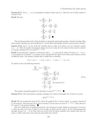
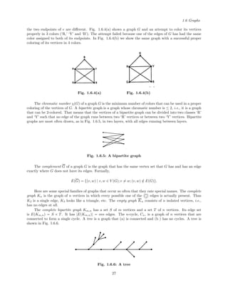
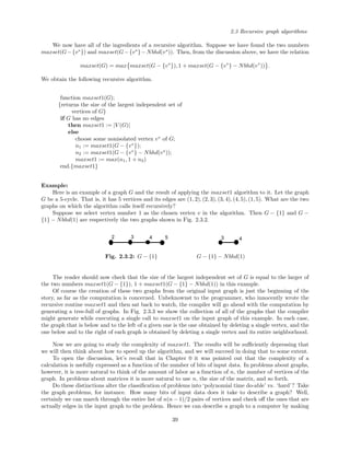
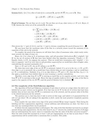
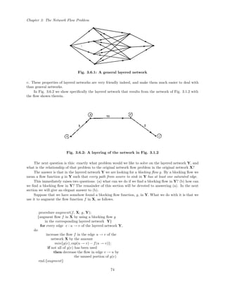
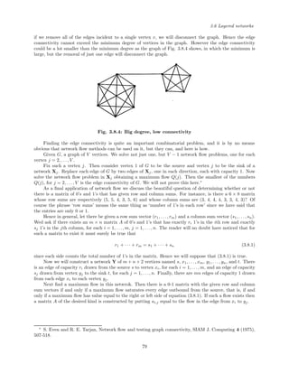
We will now prove the correctness of split.
Theorem 2.2.1. Procedure split correctly splits the array x around the chosen value T.
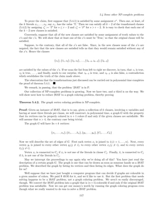
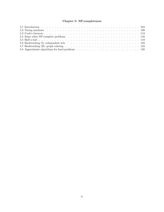
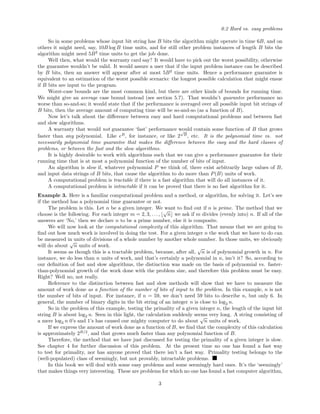
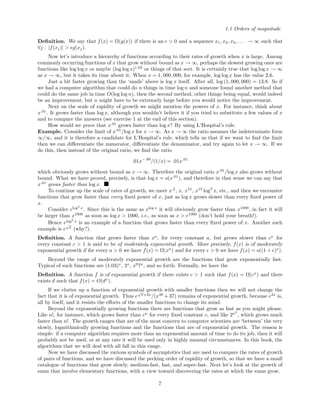
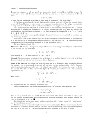
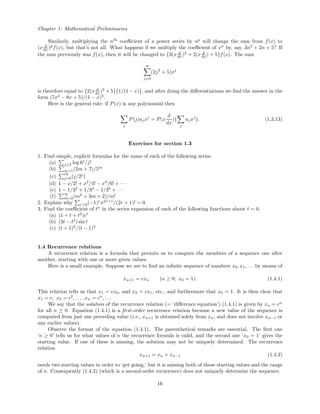
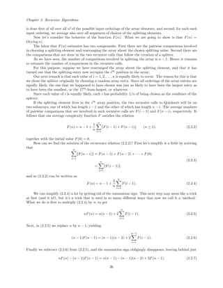
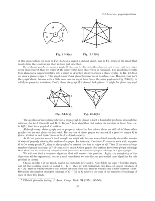
Proof: We claim that as the loop in lines 7 and 8 is repeatedly executed for j := left + 1 to right, the
following three assertions will always be true just after each execution of lines 7, 8:
(a) x[left] = T and
(b) x[r] < T for all left < r ≤ i and
(c) x[r] ≥ T for all i < r ≤ j
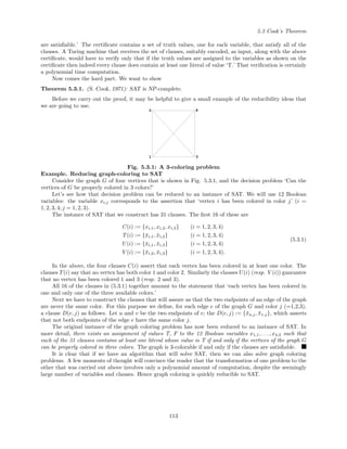
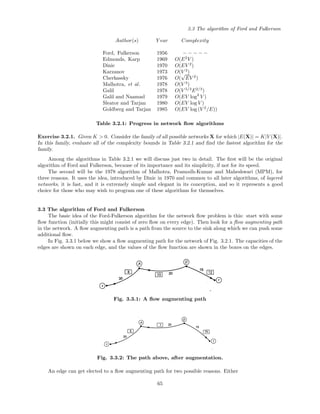
Fig. 2.2.1 illustrates the claim.
Fig. 2.2.1: Conditions (a), (b), (c)
To see this, observe first that (a), (b), (c) are surely true at the beginning, when j = left + 1. Next, if
for some j they are true, then the execution of lines 7, 8 guarantee that they will be true for the next value
of j.
Now look at (a), (b), (c) when j = right. It tells us that just prior to the execution of line 9 the
condition of the array will be
(a) x[left] = T and
(b) x[r] < T for all left < r ≤ i and
(c) x[r] ≥ T for all i < r ≤ right.
When line 9 executes, the array will be in the correctly split condition.
Now we can state a ‘final’ version of qksort (and therefore of Quicksort too).
34](https://image.slidesharecdn.com/algorithmsandcomplexity-160122031826/85/Algorithms-andcomplexity-38-320.jpg)
![2.2 Quicksort
procedure qksort(x:array; left, right:integer);
{sorts the subarray x[left], . . . , x[right]};
if right − left ≥ 1 then
split(x, left, right, i);
qksort(x, left, i − 1);
qksort(x, i + 1, right)
end.{qksort}
procedure Quicksort(x :array; n:integer)
{sorts an array of length n};
qksort(x, 1, n)
end.{Quicksort}
Now let’s consider the complexity of Quicksort. How long does it take to sort an array? Well, the
amount of time will depend on exactly which array we happen to be sorting, and furthermore it will depend
on how lucky we are with our random choices of splitting elements.
If we want to see Quicksort at its worst, suppose we have a really unlucky day, and that the random
choice of the splitter element happens to be the smallest element in the array. Not only that, but suppose
this kind of unlucky choice is repeated on each and every recursive call.
If the splitter element is the smallest array entry, then it won’t do a whole lot of splitting. In fact, if
the original array had n entries, then one of the two recursive calls will be to an array with no entries at all,
and the other recursive call will be to an array of n − 1 entries. If L(n) is the number of paired comparisons
that are required in this extreme scenario, then, since the number of comparisons that are needed to carry
out the call to split an array of length n is n − 1, it follows that
L(n) = L(n − 1) + n − 1 (n ≥ 1; L(0) = 0).
Hence,
L(n) = (1 + 2 + · · · + (n − 1)) = Θ(n2
).
The worst-case behavior of Quicksort is therefore quadratic in n. In its worst moods, therefore, it is as bad
as ‘slowsort’ above.
Whereas the performance of slowsort is pretty much always quadratic, no matter what the input is,
Quicksort is usually a lot faster than its worst case discussed above.
We want to show that on the average the running time of Quicksort is O(n log n).
The first step is to get quite clear about what the word ‘average’ refers to. We suppose that the entries
of the input array x are all distinct. Then the performance of Quicksort can depend only on the sequence of
size relationships in the input array and the choices of the random splitting elements.
The actual numerical values that appear in the input array are not in themselves important, except that,
to simplify the discussion we will assume that they are all different. The only thing that will matter, then,
will be the set of outcomes of all of the paired comparisons of two elements that are done by the algorithm.
Therefore, we will assume, for the purposes of analysis, that the entries of the input array are exactly the
set of numbers 1, 2, . . . , n in some order.
There are n! possible orders in which these elements might appear, so we are considering the action of
Quicksort on just these n! inputs.
Second, for each particular one of these inputs, the choices of the splitting elements will be made by
choosing, at random, one of the entries of the array at each step of the recursion. We will also average over
all such random choices of the splitting elements.
Therefore, when we speak of the function F(n), the average complexity of Quicksort, we are speaking of
the average number of pairwise comparisons of array entries that are made by Quicksort, where the averaging
35](https://image.slidesharecdn.com/algorithmsandcomplexity-160122031826/85/Algorithms-andcomplexity-39-320.jpg)
![2.2 Quicksort
After some tidying up, (2.2.7) becomes
F(n) = (1 +
1
n
)F(n − 1) + (2 −
2
n
). (2.2.8)
which is exactly in the form of the general first-order recurrence relation that we discussed in section 1.4.
In section 1.4 we saw that to solve (2.2.8) the winning tactic is to change to a new variable yn that is
defined, in this case, by
F(n) =
n + 1
n
n
n − 1
n − 1
n − 2
· · ·
2
1
yn
= (n + 1)yn.
(2.2.9)
If we make the change of variable F(n) = (n + 1)yn in (2.2.8), then it takes the form
yn = yn−1 + 2(n − 1)/n(n + 1) (n ≥ 1) (2.2.10)
as an equation for the yn’s (y0 = 0).
The solution of (2.2.10) is obviously
yn = 2
n
j=1
j − 1
j(j + 1)
= 2
n
j=1
{
2
j + 1
−
1
j
}
= 2
n
j=1
1
j
− 4n/(n + 1).
Hence from (2.2.9),
F(n) = 2(n + 1){
n
j=1
1/j} − 4n (2.2.11)
is the average number of pairwise comparisons that we do if we Quicksort an array of length n. Evidently
F(n) ∼ 2n log n (n → ∞) (see (1.1.7) with g(t) = 1/t), and we have proved
Theorem 2.2.2. The average number of pairwise comparisons of array entries that Quicksort makes when
it sorts arrays of n elements is exactly as shown in (2.2.11), and is ∼ 2n log n (n → ∞).
Quicksort is, on average, a very quick sorting method, even though its worst case requires a quadratic
amount of labor.
Exercises for section 2.2
1. Write out an array of 10 numbers that contains no splitter. Write out an array of 10 numbers that
contains 10 splitters.
2. Write a program that does the following. Given a positive integer n. Choose 100 random permutations
of [1, 2, . . . , n],* and count how many of the 100 had at least one splitter. Execute your program for n =
5, 6, . . . , 12 and tabulate the results.
3. Think of some method of sorting n numbers that isn’t in the text. In the worst case, how many comparisons
might your method do? How many swaps?
* For a fast and easy way to do this see A. Nijenhuis and H. S. Wilf, Combinatorial Algorithms, 2nd ed. (New
York: Academic Press, 1978), chap. 6.
37](https://image.slidesharecdn.com/algorithmsandcomplexity-160122031826/85/Algorithms-andcomplexity-41-320.jpg)
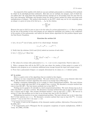
![Chapter 2: Recursive Algorithms
The Fourier transform moves us from coefficients to values at roots of unity. Some good reasons for
wanting to make that trip will appear presently, but for the moment, let’s consider the computational side
of the question, namely how to compute the Fourier transform efficiently.
We are going to derive an elegant and very speedy algorithm for the evaluation of Fourier transforms.
The algorithm is called the Fast Fourier Transform (FFT) algorithm. In order to appreciate how fast it is,
let’s see how long it would take us to calculate the transform without any very clever procedure.
What we have to do is to compute the values of a given polynomial at n given points. How much work
is required to calculate the value of a polynomial at one given point? If we want to calculate the value of
the polynomial x0 + x1t + x2t2
+ . . . + xn−1tn−1
at exactly one value of t, then we can do (think how you
would do it, before looking)
function value(x :coeff array; n:integer; t:complex);
{computes value := x0 + x1t + · · · + xn−1tn−1
}
value := 0;
for j := n − 1 to 0 step −1 do
value := t · value + xj
end.{value}
This well-known algorithm (= ‘synthetic division’) for computing the value of a polynomial at a single
point t obviously runs in time O(n).
If we calculate the Fourier transform of a given sequence of n points by calling the function value n
times, once for each point of evaluation, then obviously we are looking at a simple algorithm that requires
Θ(n2
) time.
With the FFT we will see that the whole job can be done in time O(n log n), and we will then look
at some implications of that fact. To put it another way, the cost of calculating all n of the values of a
polynomial f at the nth
roots of unity is much less than n times the cost of one such calculation.
First we consider the important case where n is a power of 2, say n = 2r
. Then the values of f, a
polynomial of degree 2r
− 1, at the (2r
)th
roots of unity are, from (2.5.6),
f(ωj) =
n−1
k=0
xkexp{2πijk/2r
} (j = 0, 1, . . . , 2r
− 1). (2.5.7)
Let’s break up the sum into two sums, containing respectively the terms where k is even and those where k
is odd. In the first sum write k = 2m and in the second put k = 2m + 1. Then, for each j = 0, 1, . . ., 2r
− 1,
f(ωj) =
2r−1
−1
m=0
x2me2πijm/2r−1
+
2r−1
−1
m=0
x2m+1e2πij(2m+1)/2r
=
2r−1
−1
m=0
x2me2πijm/2r−1
+ e2πij/2r
2r−1
−1
m=0
x2m+1e2πijm/2r−1
.
(2.5.8)
Something special just happened. Each of the two sums that appear in the last member of (2.5.8) is
itself a Fourier transform, of a shorter sequence. The first sum is the transform of the array
x[0], x[2], x[4], . . . , x[2r
− 2] (2.5.9)
and the second sum is the transform of
x[1], x[3], x[5], . . . , x[2r
− 1]. (2.5.10)
The stage is set (well, almost set) for a recursive program.
52](https://image.slidesharecdn.com/algorithmsandcomplexity-160122031826/85/Algorithms-andcomplexity-56-320.jpg)
![2.5 The discrete Fourier transform
There is one small problem, though. In (2.5.8) we want to compute f(ωj) for 2r
values of j, namely for
j = 0, 1, . . ., 2r
− 1. However, the Fourier transform of the shorter sequence (2.5.9) is defined for only 2r−1
values of j, namely for j = 0, 1, . . . , 2r−1
− 1. So if we calculate the first sum by a recursive call, then we
will need its values for j’s that are outside the range for which it was computed.
This problem is no sooner recognized than solved. Let Q(j) denote the first sum in (2.5.8). Then we
claim that Q(j) is a periodic function of j, of period 2r−1
, because
Q(j + 2r−1
) =
2r−1
−1
m=0
x2mexp{2πim(j + 2r−1
)/2r−1
}
=
2r−1
−1
m=0
x2mexp{2πimj/2r−1
}e2πim
=
2r−1
−1
m=0
x2mexp{2πimj/2r−1
}
= Q(j)
(2.5.11)
for all integers j. If Q(j) has been computed only for 0 ≤ j ≤ 2r−1
− 1 and if we should want its value for
some j ≥ 2r−1
then we can get that value by asking for Q(j mod 2r−1
).
Now we can state the recursive form of the Fast Fourier Transform algorithm in the (most important)
case where n is a power of 2. In the algorithm we will use the type complexarray to denote an array of
complex numbers.
function FFT(n:integer; x :complexarray):complexarray;
{computes fast Fourier transform of n = 2k
numbers x }
if n = 1 then FFT[0] := x[0]
else
evenarray := {x[0], x[2], . . . , x[n − 2]};
oddarray := {x[1], x[3], . . . , x[n − 1]};
{u[0], u[1], . . .u[n
2 − 1]} := FFT(n/2, evenarray);
{v[0], v[1], . . . v[n
2 − 1]} := FFT(n/2, oddarray);
for j := 0 to n − 1 do
τ := exp{2πij/n};
FFT[j] := u[j mod n
2 ] + τv[j mod n
2 ]
end.{FFT}
Let y(k) denote the number of multiplications of complex numbers that will be done if we call FFT on
an array whose length is n = 2k
. The call to FFT(n/2, evenarray) costs y(k − 1) multiplications as does
the call to FFT(n/2, oddarray). The ‘for j:= 0 to n’ loop requires n more multiplications. Hence
y(k) = 2y(k − 1) + 2k
(k ≥ 1; y(0) = 0). (2.5.12)
If we change variables by writing y(k) = 2k
zk, then we find that zk = zk−1 + 1, which, together with z0 = 0,
implies that zk = k for all k ≥ 0, and therefore that y(k) = k2k
. This proves
Theorem 2.5.1. The Fourier transform of a sequence of n complex numbers is computed using only
O(n log n) multiplications of complex numbers by means of the procedure FFT, if n is a power of 2.
Next* we will discuss the situation when n is not a power of 2.
The reader may observe that by ‘padding out’ the input array with additional 0’s we can extend the
length of the array until it becomes a power of 2, and then call the FFT procedure that we have already
* The remainder of this section can be omitted at a first reading.
53](https://image.slidesharecdn.com/algorithmsandcomplexity-160122031826/85/Algorithms-andcomplexity-57-320.jpg)
![2.5 The discrete Fourier transform
computation, hence all of the necessary values of ak(j) can be found with r1g(r2) complex multiplications.
Once the ak(j) are all in hand, then the computation of the one value of the transform from (2.5.13) will
require an additional r1 − 1 complex multiplications. Since n = r1r2 values of the transform have to be
computed, we will need r1r2(r1 − 1) complex multiplications.
The complete computation needs r1g(r2) + r2
1r2 − r1r2 multiplications if we choose a particular factor-
ization n = r1r2. The factorization that should be chosen is the one that minimizes the labor, so we have
the recurrence
g(n) = min
n=r1r2
{r1g(r2) + r2
1r2} − n. (2.5.16)
If n = p is a prime number then there are no factorizations to choose from and our algorithm is no help
at all. There is no recourse but to calculate the p values of the transform directly from the definition (2.5.6),
and that will require p − 1 complex multiplications to be done in order to get each of those p values. Hence
we have, in addition to the recurrence formula (2.5.16), the special values
g(p) = p(p − 1) (if p is prime). (2.5.17)
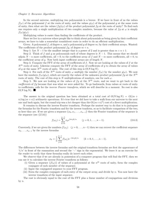
The recurrence formula (2.5.16) together with the starting values that are shown in (2.5.17) completely
determine the function g(n). Before proceeding, the reader is invited to calculate g(12) and g(18).
We are going to work out the exact solution of the interesting recurrence (2.5.16), (2.5.17), and when
we are finished we will see which factorization of n is the best one to choose. If we leave that question in
abeyance for a while, though, we can summarize by stating the (otherwise) complete algorithm for the fast
Fourier transform.
function FFT(x:complexarray; n:integer):complexarray;
{computes Fourier transform of a sequence x of length n}
if n is prime
then
for j:=0 to n − 1 do
FFT[j] := n−1
k=0 x[k]ξn
jk
else
let n = r1r2 be some factorization of n;
{see below for best choice of r1, r2}
for k:=0 to r1 − 1 do
{ak[0], ak[1], . . . , ak[r2 − 1]}
:= FFT({x[k], x[k + r1], . . . , x[k + (r2 − 1)r1]}, r2);
for j:=0 to n − 1 do
FFT[j] := r1−1
k=0 ak[j mod r2]ξkj
n
end.{FFT}
Our next task will be to solve the recurrence relations (2.5.16), (2.5.17), and thereby to learn the best
choice of the factorization of n.
Let g(n) = nh(n), where h is a new unknown function. Then the recurrence that we have to solve takes
the form
h(n) =
mind{h(n/d) + d} − 1, if n is composite;
n − 1, if n is prime.
(2.5.18)
In (2.5.18), the ‘min’ is taken over all d that divide n other than d = 1 and d = n.
The above relation determines the value of h for all positive integers n. For example,
h(15) = min
d
(h(15/d) + d) − 1
= min(h(5) + 3, h(3) + 5) − 1
= min(7, 7) − 1 = 6
55](https://image.slidesharecdn.com/algorithmsandcomplexity-160122031826/85/Algorithms-andcomplexity-59-320.jpg)
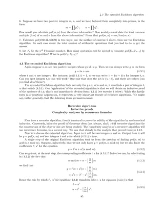
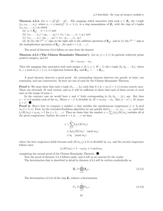
![Chapter 4: Algorithms in the Theory of Numbers
The reader should now review the discussion in Example 3 of section 0.2. In that example we showed
that the obvious methods of testing for primality are slow in the sense of complexity theory. That is, we
do an amount of work that is an exponentially growing function of the length of the input bit string if we
use one of those methods. So this problem, which seems like a ‘pushover’ at first glance, turns out to be
extremely difficult.
Although it is not known if a polynomial-time primality testing algorithm exists, remarkable progress
on the problem has been made in recent years.
One of the most important of these advances was made independently and almost simultaneously by
Solovay and Strassen, and by Rabin, in 1976-7. These authors took the imaginative step of replacing
‘certainly’ by ‘probably,’ and they devised what should be called a probabilistic compositeness (an integer
is composite if it is not prime) test for integers, that runs in polynomial time.
Here is how the test works. First choose a number b uniformly at random, 1 ≤ b ≤ n − 1. Next,
subject the pair (b, n) to a certain test, called a pseudoprimality test, to be described below. The test has
two possible outcomes: either the number n is correctly declared to be composite or the test is inconclusive.
If that were the whole story it would be scarcely have been worth the telling. Indeed the test ‘Does b
divide n?’ already would perform the function stated above. However, it has a low probability of success
even if n is composite, and if the answer is ‘No,’ we would have learned virtually nothing.
The additional property that the test described below has, not shared by the more naive test ‘Does b
divide n?,’ is that if n is composite, the chance that the test will declare that result is at least 1/2.
In practice, for a given n we would apply the test 100 times using 100 numbers bi that are independently
chosen at random in [1, n − 1]. If n is composite, the probability that it will be declared composite at least
once is at least 1−2−100
, and these are rather good odds. Each test would be done in quick polynomial time.
If n is not found to be composite after 100 trials, and if certainty is important, then it would be worthwhile
to subject n to one of the nonprobabilistic primality tests in order to dispel all doubt.
It remains to describe the test to which the pair (b, n) is subjected, and to prove that it detects com-
positeness with probability ≥ 1/2.
Before doing this we mention another important development. A more recent primality test, due to
Adleman, Pomerance and Rumely in 1983, is completely deterministic. That is, given n it will surely decide
whether or not n is prime. The test is more elaborate than the one that we are about to describe, and it
runs in tantalizingly close to polynomial time. In fact it was shown to run in time
O((log n)c log log log n
)
for a certain constant c. Since the number of bits of n is a constant multiple of log n, this latter estimate is
of the form
O((Bits)c log log Bits
).
The exponent of ‘Bits,’ which would be constant in a polynomial time algorithm, in fact grows extremely
slowly as n grows. This is what was referred to as ‘tantalizingly close’ to polynomial time, earlier.
It is important to notice that in order to prove that a number is not prime, it is certainly sufficient to
find a nontrivial divisor of that number. It is not necessary to do that, however. All we are asking for is a
‘yes’ or ‘no’ answer to the question ‘is n prime?.’ If you should find it discouraging to get only the answer
‘no’ to the question ‘Is 7122643698294074179 prime?,’ without getting any of the factors of that number,
then what you want is a fast algorithm for the factorization problem.
In the test that follows, the decision about the compositeness of n will be reached without a knowledge
of any of the factors of n. This is true of the Adleman, Pomerance, Rumely test also. The question of
finding a factor of n, or all of them, is another interesting computational problem that is under active
investigation. Of course the factorization problem is at least as hard as finding out if an integer is prime,
and so no polynomial-time algorithm is known for it either. Again, there are probabilistic algorithms for the
factorization problem just as there are for primality testing, but in the case of the factorization problem,
even they don’t run in polynomial-time.
In section 4.9 we will discuss a probabilistic algorithm for factoring large integers, after some motivation
in section 4.8, where we remark on the connection between computationally intractable problems and cryp-
tography. Specifically, we will describe one of the ‘Public Key’ data encryption systems whose usefulness
stems directly from the difficulty of factoring large integers.
88](https://image.slidesharecdn.com/algorithmsandcomplexity-160122031826/85/Algorithms-andcomplexity-92-320.jpg)
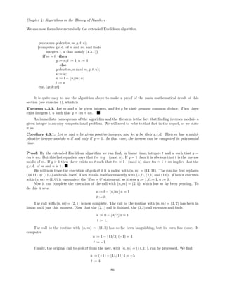
![Chapter 4: Algorithms in the Theory of Numbers
of the group of units. Since Un is a group, (4.5.3) is an isomorphism of the multiplicative structure only. In
Z12, for example, we find
U12
∼= U4U3
where U4 = {1, 3}, U3 = {1, 2}. So U12 can be thought of as the set {(1, 1, ), (1, 2), (3, 1), (3, 2)}, together
with the componentwise multiplication operation described above.
Exercises for section 4.5
1. Give a complete proof of theorem 4.5.4.
2. Find all primitive roots modulo 18.
3. Find all primitive roots modulo 27.
4. Write out the multiplication table of the group U27.
5. Which elements of Z11 are squares?
6. Which elements of Z13 are squares?
7. Find all x ∈ U27 such that x2
= 1. Find all x ∈ U15 such that x2
= 1.
8. Prove that if there is a primitive root modulo n then the equation x2
= 1 in the group Un has only the
solutions x = ±1.
9. Find a number x that is congruent to 1, 7 and 11 to the respective moduli 5, 11 and 17. Use the method
in the second proof of the remainder theorem 4.5.5.
10. Write out the complete proof of the ‘immediate’ corollary 4.5.3.
4.6 Pseudoprimality tests
In this section we will discuss various tests that might be used for testing the compositeness of integers
probabilistically.
By a pseudoprimality test we mean a test that is applied to a pair (b, n) of integers, and that has the
following characteristics:
(a) The possible outcomes of the test are ‘n is composite’ or ‘inconclusive.’
(b) If the test reports ‘n is composite’ then n is composite.
(c) The test runs in a time that is polynomial in logn.
If the test result is ‘inconclusive’ then we say that n is pseudoprime to the base b (which means that n
is so far acting like a prime number, as far as we can tell).
The outcome of the test of the primality of n depends on the base b that is chosen. In a good pseu-
doprimality test there will be many bases b that will give the correct answer. More precisely, a good
pseudoprimality test will, with high probability (i.e., for a large number of choices of the base b) declare
that a composite n is composite. In more detail, we will say that a pseudoprimality test is ‘good’ if there
is a fixed positive number t such that every composite integer n is declared to be composite for at least tn
choices of the base b, in the interval 1 ≤ b ≤ n.
Of course, given an integer n, it is silly to say that ‘there is a high probability that n is prime.’ Either
n is prime or it isn’t, and we should not blame our ignorance on n itself. Nonetheless, the abuse of language
is sufficiently appealing that we will define the problem away: we will say that a given integer n is very
probably prime if we have subjected it to a good pseudoprimality test, with a large number of different bases
b, and have found that it is pseudoprime to all of those bases.
Here are four examples of pseudoprimality tests, only one of which is ‘good.’
Test 1. Given b, n. Output ‘n is composite’ if b divides n, else ‘inconclusive.’
This isn’t the good one. If n is composite, the probability that it will be so declared is the probability
that we happen to have found a b that divides n, where b is not 1 or n. The probability of this event, if b is
chosen uniformly at random from [1, n], is
p1 = (d(n) − 2)/n
where d(n) is the number of divisors of n. Certainly p1 is not bounded from below by a positive constant t,
if n is composite.
92](https://image.slidesharecdn.com/algorithmsandcomplexity-160122031826/85/Algorithms-andcomplexity-96-320.jpg)
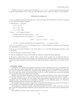
![4.6 Pseudoprimality tests
Test 2. Given b, n. Output ‘n is composite’ if gcd(b, n) = 1, else output ‘inconclusive.’
This one is a little better, but not yet good. If n is composite, the number of bases b ≤ n for which
Test 2 will produce the result ‘composite’ is n − φ(n), where φ is the Euler totient function, of (4.1.5). This
number of useful bases will be large if n has some small prime factors, but in that case it’s easy to find
out that n is composite by other methods. If n has only a few large prime factors, say if n = p2
, then the
proportion of useful bases is very small, and we have the same kind of inefficiency as in Test 1 above.
Now we can state the third pseudoprimality test.
Test 3. Given b, n. (If b and n are not relatively prime or) if bn−1
≡ 1 (mod n) then output ‘n is
composite,’ else output ‘inconclusive.’
Regrettably, the test is still not ‘good,’ but it’s a lot better than its predecessors. To cite an extreme
case of its un-goodness, there exist composite numbers n, called Carmichael numbers, with the property that
the pair (b, n) produces the output ‘inconclusive’ for every integer b in [1, n − 1] that is relatively prime to
n. An example of such a number is n = 1729, which is composite (1729 = 7 · 13 · 19), but for which Test
3 gives the result ‘inconclusive’ on every integer b < 1729 that is relatively prime to 1729 (i.e., that is not
divisible by 7 or 13 or 19).
Despite such misbehavior, the test usually seems to perform quite well. When n = 169 (a difficult
integer for tests 1 and 2) it turns out that there are 158 different b’s in [1,168] that produce the ‘composite’
outcome from Test 3, namely every such b except for 19, 22, 23, 70, 80, 89, 99, 146, 147, 150, 168.
Finally, we will describe a good pseudoprimality test. The familial resemblance to Test 3 will be
apparent.
Test 4. (the strong pseudoprimality test): Given (b, n). Let n − 1 = 2q
m, where m is an odd integer. If
either
(a) bm
≡ 1 (mod n) or
(b) there is an integer i in [0, q − 1] such that
bm2i
≡ −1 (mod n)
then return ‘inconclusive’ else return ‘n is composite.’
First we validate the test by proving the
Proposition. If the test returns the message ‘n is composite,’ then n is composite.
Proof: Suppose not. Then n is an odd prime. We claim that
bm2i
≡ 1 (mod n)
for all i = q, q − 1, . . . , 0. If so then the case i = 0 will contradict the outcome of the test, and thereby
complete the proof. To establish the claim, it is clearly true when i = q, by Fermat’s theorem. If true for i,
then it is true for i − 1 also, because
(bm2i−1
)2
= bm2i
≡ 1 (mod n)
implies that the quantity being squared is +1 or −1. Since n is an odd prime, by corollary 4.5.3 Un is cyclic,
and so the equation x2
= 1 in Un has only the solutions x = ±1. But −1 is ruled out by the outcome of the
test, and the proof of the claim is complete.
What is the computational complexity of the test? Consider first the computational problem of raising
a number to a power. We can calculate, for example, bm
mod n with O(log m) integer multiplications,
by successive squaring. More precisely, we compute b, b2
, b4
, b8
, . . . by squaring, and reducing modulo n
immediately after each squaring operation, rather than waiting until the final exponent is reached. Then we
use the binary expansion of the exponent m to tell us which of these powers of b we should multiply together
in order to compute bm
. For instance,
b337
= b256
· b64
· b16
· b.
93](https://image.slidesharecdn.com/algorithmsandcomplexity-160122031826/85/Algorithms-andcomplexity-97-320.jpg)
![Chapter 4: Algorithms in the Theory of Numbers
The complete power algorithm is recursive and looks like this:
function power(b, m, n);
{returns bm
mod n}
if m = 0
then
power := 1
else
t := sqr(power(b, m/2 , n));
if m is odd then t := t · b;
power := t mod n
end.{power}
Hence part (a) of the strong pseudoprimality test can be done in O(log m) = O(log n) multiplications
of integers of at most O(log n) bits each. Similarly, in part (b) of the test there are O(log n) possible values
of i to check, and for each of them we do a single multiplication of two integers each of which has O(log n)
bits (this argument, of course, applies to Test 3 above also).
The entire test requires, therefore, some low power of logn bit operations. For instance, if we were to
use the most obvious way to multiply two B bit numbers we would do O(B2
) bit operations, and then the
above test would take O((log n)3
) time. This is a polynomial in the number of bits of input.
In the next section we are going to prove that Test 4 is a good pseudoprimality test in that if n is
composite then at least half of the integers b, 1 ≤ b ≤ n − 1 will give the result ‘n is composite.’
For example, if n = 169, then it turns out that for 157 of the possible 168 bases b in [1,168], Test 4 will
reply ‘169 is composite.’ The only bases b that 169 can fool are 19, 22, 23, 70, 80, 89, 99, 146, 147, 150,
168. For this case of n = 169 the performances of Test 4 and of Test 3 are identical. However, there are no
analogues of the Carmichael numbers for Test 4.
Exercises for section 4.6
1. Given an odd integer n. Let T(n) be the set of all b ∈ [1, n] such that gcd(b, n) = 1 and bn−1
≡ 1
(mod n). Show that |T(n)| divides φ(n).
2. Let H be a cyclic group of order n. How many elements of each order r are there in H (r divides n)?
3. If n = pa
, where p is an odd prime, then the number of x ∈ Un such that x has exact order r, is φ(r), for
all divisors r of φ(n). In particular, the number of primitive roots modulo n is φ(φ(n)).
4. If n = pa1
1 · · · pam
m , and if r divides φ(n), then the number of x ∈ Un such that xr
≡ 1 (mod n) is
m
i=1
gcd(φ(pai
i ), r).
5. In a group G suppose fm and gm are, respectively, the number of elements of order m and the number
of solutions of the equation xm
= 1, for each m = 1, 2, . . .. What is the relationship between these two
sequences? That is, how would you compute the g’s from the f’s? the f’s from the g’s? If you have never
seen a question of this kind, look in any book on the theory of numbers, find ‘M¨obius inversion,’ and apply
it to this problem.
4.7 Proof of goodness of the strong pseudoprimality test
In this section we will show that if n is composite, then at least half of the integers b in [1, n − 1] will
yield the result ‘n is composite’ in the strong pseudoprimality test. The basic idea of the proof is that a
subgroup of a group that is not the entire group can consist of at most half of the elements of that group.
Suppose n has the factorization
n = pa1
1 · · · pas
s
and let ni = pi
ai
(i = 1, s).
94](https://image.slidesharecdn.com/algorithmsandcomplexity-160122031826/85/Algorithms-andcomplexity-98-320.jpg)
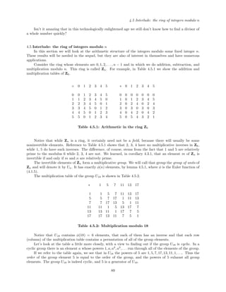
![4.7 Goodness of pseudoprimality test
Lemma 4.7.1. The order of each element of Un is a divisor of e∗
= lcm{φ(ni); i = 1, s}.
Proof: From the product representation (4.5.3) of Un we find that an element x of Un can be regarded as
an s-tuple of elements from the cyclic groups Uni (i = 1, s). The order of x is equal to the lcm of the orders
of the elements of the s-tuple. But for each i = 1, . . . , s the order of the ith
of those elements is a divisor of
φ(ni), and therefore the order of x divides the lcm shown above.
Lemma 4.7.2. Let n > 1 be odd. For each element u of Un let C(u) = {1, u, u2
, . . . , ue−1
} denote the cyclic
group that u generates. Let B be the set of all elements u of Un for which C(u) either contains −1 or has
odd order (e odd). If B generates the full group Un then n is a prime power.
Proof: Let e∗
= 2t
m, where m is odd and e∗
is as shown in lemma 4.7.1. Then there is a j such that φ(nj)
is divisible by 2t
.
Now if n is a prime power, we are finished. So we can suppose that n is divisible by more than one
prime number. Since φ(n) is an even number for all n > 2 (proof?), the number e∗
is even. Hence t > 0 and
we can define a mapping ψ of the group Un to itself by
ψ(x) = x2t−1
m
(x ∈ Un)
(note that ψ(x) is its own inverse).
This is in fact a group homomorphism:
∀x, y ∈ Un : ψ(xy) = ψ(x)ψ(y).
Let B be as in the statement of lemma 4.7.2. For each x ∈ B, ψ(x) is in C(x) and
ψ(x)2
= ψ(x2
) = 1.
Since ψ(x) is an element of C(x) whose square is 1, ψ(x) has order 1 or 2. Hence if ψ(x) = 1, it is of order
2. If the cyclic group C(x) is of odd order then it contains no element of even order. Hence C(x) is of even
order and contains −1. Then it can contain no other element of order 2, so ψ(x) = −1 in this case.
Hence for every x ∈ B, ψ(x) = ±1.
Suppose B generates the full group Un. Then not only for every x ∈ B but for every x ∈ Un it is true
that ψ(x) = ±1.
Suppose n is not a prime power. Then s > 1 in the factorization (4.5.2) of Un. Consider the element v
of Un which, when written out as an s-tuple according to that factorization, is of the form
v = (1, 1, 1, . . ., 1, y, 1, . . ., 1)
where the ‘y’ is in the jth
component, y ∈ Unj (recall that j is as described above, in the second sentence of
this proof). We can suppose y to be an element of order exactly 2t
in Unj since Unj is cyclic.
Consider ψ(v). Clearly ψ(v) is not 1, for otherwise the order of y, namely 2t
, would divide 2t−1
m, which
is impossible because m is odd.
Also, ψ(v) is not −1, because the element −1 of Un is represented uniquely by the s-tuple all of whose
entries are −1. Thus ψ(v) is neither 1 nor −1 in Un, which contradicts the italicized assertion above. Hence
s = 1 and n is a prime power, completing the proof.
Now we can prove the main result of Solovay, Strassen and Rabin, which asserts that Test 4 is good.
Theorem 4.7.1. Let B be the set of integers b mod n such that (b, n) returns ‘inconclusive’ in Test 4.
(a) If B generates Un then n is prime.
(b) If n is composite then B consists of at most half of the integers in [1, n − 1].
Proof: Suppose b ∈ B and let m be the odd part of n − 1. Then either bm
≡ 1 or bm2i
≡ −1 for some
i ∈ [0, q − 1]. In the former case the cyclic subgroup C(b) has odd order, since m is odd, and in the latter
case C(b) contains −1.
95](https://image.slidesharecdn.com/algorithmsandcomplexity-160122031826/85/Algorithms-andcomplexity-99-320.jpg)
![Chapter 4: Algorithms in the Theory of Numbers
Hence in either case B ⊆ B, where B is the set defined in the statement of lemma 4.7.2 above. If B
generates the full group Un then B does too, and by lemma 4.7.2, n is a prime power, say n = pk
.
Also, in either of the above cases we have bn−1
≡ 1, so the same holds for all b ∈ B , and so for all
x ∈ Un we have xn−1
≡ 1, since B generates Un.
Now Un is cyclic of order
φ(n) = φ(pk
) = pk−1
(p − 1).
By theorem 4.5.3 there are primitive roots modulo n = pk
. Let g be one of these. The order of g is, on the
one hand, pk−1
(p−1) since the set of all of its powers is identical with Un, and on the other hand is a divisor
of n − 1 = pk
− 1 since xn−1
≡ 1 for all x, and in particular for x = g.
Hence pk−1
(p − 1) (which, if k > 1, is a multiple of p) divides pk
− 1 (which is one less than a multiple
of p), and so k = 1, which completes the proof of part (a) of the theorem.
In part (b), n is composite and so B cannot generate all of Un, by part (a). Hence B generates a
proper subgroup of Un, and so can contain at most half as many elements as Un contains, and the proof is
complete.
Another application of the same circle of ideas to computer science occurs in the generation of random
numbers on a computer. A good way to do this is to choose a primitive root modulo the word size of your
computer, and then, each time the user asks for a random number, output the next higher power of the
primitive root. The fact that you started with a primitive root insures that the number of ‘random numbers’
generated before repetition sets in will be as large as possible.
Now we’ll summarize the way in which the primality test is used. Suppose there is given a large integer
n, and we would like to determine if it is prime.
We would do
function testn(n, outcome);
times := 0;
repeat
choose an integer b uniformly at random in [2, n − 1];
apply the strong pseudoprimality test (Test 4) to the
pair (b, n);
times := times + 1
until {result is ‘n is composite’ or times = 100};
if times = 100 then outcome:=‘n probably prime’
else outcome:=‘n is composite’
end{testn}
If the procedure exits with ‘n is composite,’ then we can be certain that n is not prime. If we want to
see the factors of n then it will be necessary to use some factorization algorithm, such as the one described
below in section 4.9.
On the other hand, if the procedure halts because it has been through 100 trials without a conclusive
result, then the integer n is very probably prime. More precisely, the chance that a composite integer n
would have behaved like that is less than 2−100
. If we want certainty, however, it will be necessary to apply a
test whose outcome will prove primality, such as the algorithm of Adleman, Rumely and Pomerance, referred
to earlier.
In section 4.9 we will discuss a probabilistic factoring algorithm. Before doing so, in the next section
we will present a remarkable application of the complexity of the factoring problem, to cryptography. Such
applications remind us that primality and factorization algorithms have important applications beyond pure
mathematics, in areas of vital public concern.
Exercises for section 4.7
1. For n = 9 and for n = 15 find all of the cyclic groups C(u), of lemma 4.7.2, and find the set B.
2. For n = 9 and n = 15 find the set B , of theorem 4.7.1.
96](https://image.slidesharecdn.com/algorithmsandcomplexity-160122031826/85/Algorithms-andcomplexity-100-320.jpg)
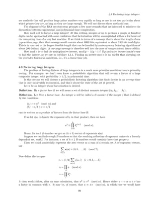
![4.8 Factoring and cryptography
4.8 Factoring and cryptography
A computationally intractable problem can be used to create secure codes for the transmission of infor-
mation over public channels of communication. The idea is that those who send the messages to each other
will have extra pieces of information that will allow the m to solve the intractable problem rapidly, whereas
an aspiring eavesdropper would be faced with an exponential amount of computation.
Even if we don’t have a provably computationally intractable problem, we can still take a chance that
those who might intercept our messages won’t know any polynomial-time algorithms if we don’t know any.
Since there are precious few provably hard problems, and hordes of apparently hard problems, it is scarcely
surprising that a number of sophisticated coding schemes rest on the latter rather than the former. One
should remember, though, that an adversary might discover fast algorithms for doing these problems and
keep that fact secret while deciphering all of our messages.
A remarkable feature of a family of recently developed coding schemes, called ‘Public Key Encryption
Systems,’ is that the ‘key’ to the code lies in the public domain, so it can be easily available to sender and
receiver (and eavesdropper), and can be readily changed if need be. On the negative side, the most widely
used Public Key Systems lean on computational problems that are only presumed to be intractable, like
factoring large integers, rather than having been proved so.
We are going to discuss a Public Key System called the RSA scheme, after its inventors: Rivest, Shamir
and Adleman. This particular method depends for its success on the seeming intractability of the problem
of finding the factors of large integers. If that problem could be done in polynomial time, then the RSA
system could be ‘cracked.’
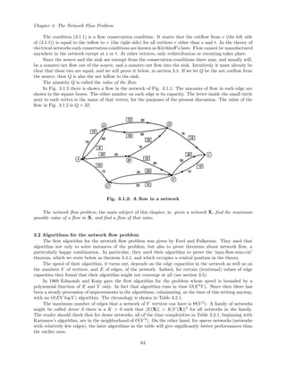
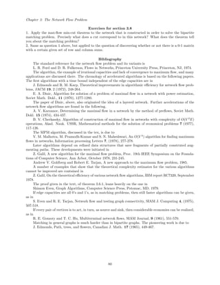
In this system there are three centers of information: the sender of the message, the receiver of the
message, and the Public Domain (for instance, the ‘Personals’ ads of the New York Times). Here is how the
system works.
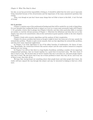
(A) Who knows what and when
Here are the items of information that are involved, and who knows each item:
p, q: two large prime numbers, chosen by the receiver, and told to nobody else (not even to the sender!).
n : the product pq is n, and this is placed in the Public Domain.
E : a random integer, placed in the Public Domain by the receiver, who has first made sure that E is
relatively prime to (p − 1)(q − 1) by computing the g.c.d., and choosing a new E at random until the g.c.d.
is 1. This is easy for the receiver to do because p and q are known to him, and the g.c.d. calculation is fast.
P : a message that the sender would like to send, thought of as a string of bits whose value, when
regarded as a binary number, lies in the range [0, n − 1].
In addition to the above, one more item of information is computed by the receiver, and that is the
integer D that is the multiplicative inverse mod (p − 1)(q − 1) of E, i.e.,
DE ≡ 1 (mod (p − 1)(q − 1)).
Again, since p and q are known, this is a fast calculation for the receiver, as we shall see.
To summarize,
The receiver knows p, q, D
The sender knows P
Everybody knows n and E
In Fig. 4.8.1 we show the interiors of the heads of the sender and receiver, as well as the contents of the
Public Domain.
97](https://image.slidesharecdn.com/algorithmsandcomplexity-160122031826/85/Algorithms-andcomplexity-101-320.jpg)
![Chapter 4: Algorithms in the Theory of Numbers
learned nothing. However if neither u ≡ v (mod n) nor u ≡ −v (mod n) is true then we will have found
a nontrivial factor of n, namely gcd(u − v, n) or gcd(u + v, n).
Example:
Take as a factor base B = {−2, 5}, and let it be required to find a factor of n = 1729. Then we claim
that 186 and 267 are B-numbers. To see that 186 is a B-number, note that 1862
= 20 · 1729 + (−2)4
, and
similarly, since 2672
= 41 · 1729 + (−2)4
52
, we see that 267 is a B-number, for this factor base B.
The exponent vectors of 186 and 167 are (4, 0) and (4, 2) respectively, and these sum to (0, 0) (mod 2),
hence we find that
u = 186 × 267 ≡ 1250 (mod 1729)
r1 = 4; r2 = 1
v = (−2)4
(5)1
= 80
gcd(u − v, n) = gcd(1170, 1729) = 13
and we have found the factor 13 of 1729.
There might have seemed to be some legerdemain involved in plucking the B-numbers 186 and 267 out
of the air, in the example above. In fact, as the algorithm has been implemented by its author, J. D. Dixon,
one simply chooses integers uniformly at random from [1, n − 1] until enough B-numbers have been found
so their exponent vectors are linearly dependent modulo 2. In Dixon’s implementation the factor base that
is used consists of −1 together with the first h prime numbers.
It can then be proved that if n is not a prime power then with a correct choice of h relative to n, if we
repeat the random choices until a factor of n is found, the average running time will be
exp{(2 + o(1))(log log log n)
.5
}.
This is not polynomial time, but it is moderately exponential only. Nevertheless, it is close to being about
the best that we know how to do on the elusive problem of factoring a large integer.
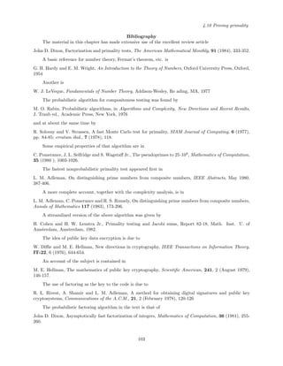
4.10 Proving primality
In this section we will consider a problem that sounds a lot like primality testing, but is really a little
different because the rules of the game are different. Basically the problem is to convince a skeptical audience
that a certain integer is prime, requiring them to do only a small amount of computation in order to be so
persuaded.
First, though, suppose you were writing a 100-decimal-digit integer n on the blackboard in front of a
large audience and you wanted to prove to them that n was not a prime.
If you simply wrote down two smaller integers whose product was n, the job would be done. Anyone
who wished to be certain could spend a few minutes multiplying the factors together and verifying that their
product was indeed n, and all doubts would be dispelled.
Indeed*, a spea ker at a mathematical convention in 1903 announced the result that 267
− 1 is not a
prime number, and to be utterly convincing all he had to do was to write
267
− 1 = 193707721 × 761838257287.
We note that the speaker probably had to work very hard to find those factors, but having found them
it became quite easy to convince others of the truth of the claimed result.
A pair of integers r, s for which r = 1, s = 1, and n = rs constitute a certificate attesting to the
compositeness of n. With this certificate C(n) and an auxiliary checking algorithm, viz.
(1) Verify that r = 1, and that s = 1
(2) Verify that rs = n
we can prove, in polynomial time, that n is not a prime number.
* We follow the account given in V. Pratt, Every prime has a succinct certificate, SIAM J. Computing, 4
(1975), 214-220.
100](https://image.slidesharecdn.com/algorithmsandcomplexity-160122031826/85/Algorithms-andcomplexity-104-320.jpg)
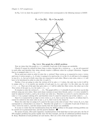
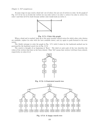
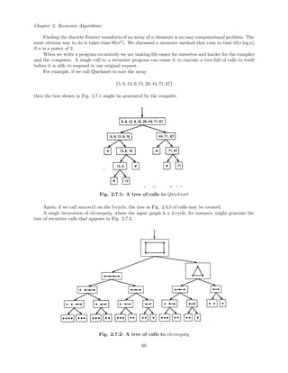
![Chapter 5: NP-completeness
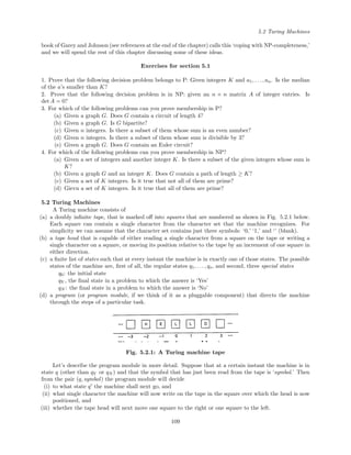
One step of the program, therefore, goes from
(state, symbol) to (newstate, newsymbol, increment). (5.2.1)
If and when the state reaches qY or qN the computation is over and the machine halts.
The machine should be thought of as part hardware and part software. The programmer’s job is, as
usual, to write the software. To write a program for a Turing machine, what we have to do is to tell it how
to make each and every one of the transitions (5.2.1). A Turing machine program looks like a table in which,
for every possible pair (state, symbol) that the machine might find itself in, the programmer has specified
what the newstate, the newsymbol and the increment shall be.
To begin a computation with a Turing machine we take the input string x, of length B, say, that describes
the problem that we want to solve, and we write x in squares 1, 2, . . ., B of the tape. The tape head is then
positioned over square 1, the machine is put into state q0, the program module that the programmer prepared
is plugged into its slot, and the computation begins.
The machine reads the symbol in square 1. It now is in state q0 and has read symbol, so it can consult
the program module to find out what to do. The program instructs it to write at square 1 a newsymbol, to
move the head either to square 0 or to square 2, and to enter a certain newstate, say q . The whole process
is then repeated, possibly forever, but hopefully after finitely many steps the machine will enter the state
qY or state qN , at which moment the computation will halt with the decision having been made.
If we want to watch a Turing machine in operation, we don’t have to build it. We can simulate one.
Here is a pidgin-Pascal simulation of a Turing machine that can easily be turned into a functioning program.
It is in two principal parts.
The procedure turmach has for input a string x of length B, and for output it sets the Boolean variable
accept to True or False, depending on whether the outcome of the computation is that the machine halted
in state qY or qN respectively. This procedure is the ‘hardware’ part of the Turing machine. It doesn’t vary
from one job to the next.
Procedure gonextto is the program module of the machine, and it will be different for each task. Its
inputs are the present state of the machine and the symbol that was just read from the tape. Its outputs
are the newstate into which the machine goes next, the newsymbol that the tape head now writes on the
current square, and the increment (±1) by which the tape head will now move.
procedure turmach(B:integer; x :array[1..B]; accept:Boolean);
{simulates Turing machine action on input string x of length B}
{write input string on tape in first B squares}
for square := 1 to B do
tape[square] :=x[square];
{record boundaries of written-on part of tape}
leftmost:=1; rightmost := B;
{initialize tape head and state}
state:=0; square:=1;
while state = ‘Y’ and state = ‘N’ do
{read symbol at current tape square}
if square< leftmost or square> rightmost
then symbol:=‘’ else symbol:= tape[square]
{ask program module for state transition}
gonnextto(state,symbol,newstate,newsybol,increment);
state:=newstate;
{update boundaries and write new symbol};
if square> rightmost then leftmost:= square;
tape[square]:=newsymbol;
{move tape head}
square := square+increment
end;{while}
accept:={ state=‘Y’}
end.{turmach}
110](https://image.slidesharecdn.com/algorithmsandcomplexity-160122031826/85/Algorithms-andcomplexity-114-320.jpg)