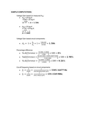
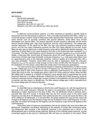
NewBase 22 April 2024 Energy News issue - 1718 by Khaled Al Awadi (AutoRe...
National College of Science and Technology Experiment No. 3
1. NATIONAL COLLEGE OF SCIENCE AND TECHNOLOGY
Amafel Building, Aguinaldo Highway Dasmariñas City, Cavite
Experiment No. 3
ACTIVE LOW-PASS and ACTIVE HIGH-PASS FILTERS
Pula, Rolando A. July 14, 2011
Signal Spectra and Signal Processing/BSECE 41A1 Score:
Engr. Grace Ramones
Instructor
2. OBJECTIVES:
1. Plot the gain-frequency response and determine the cutoff frequency of a second-order (two-
pole) low-pass active filter.
2. Plot the gain-frequency response and determine the cutoff frequency of a second-order (two-
pole) high-pass active filter.
3. Determine the roll-off in dB per decade for a second-order (two-pole) filter.
4. Plot the phase-frequency response of a second-order (two-pole) filter.
3. SAMPLE COMPUTATIONS:
Voltage Gain based on measured AdB:
AdB = 20 log A
4.006 = 20 log A
AdB = 20 log A
3.776 = 20 log A
A = 1.5445
Voltage Gain based circuit components:
Percentage difference:
Cut-off frequency based on circuit components:
4. DATA SHEET:
MATERIALS
One function generator
One dual-trace oscilloscope
One LM741 op-amp
Capacitors: two 0.001 µF, one 1 pF
Resistors: one 1kΩ, one 5.86 kΩ, two 10kΩ, two 30 kΩ
THEORY
In electronic communications systems, it is often necessary to separate a specific range of
frequencies from the total frequency spectrum. This is normally accomplished with filters. A filter is a
circuit that passes a specific range of frequencies while rejecting other frequencies. Active filters use
active devices such as op-amps combined with passive elements. Active filters have several
advantages over passive filters. The passive elements provide frequency selectivity and the active
devices provide voltage gain, high input impedance, and low output impedance. The voltage gain
reduces attenuation of the signal by the filter, the high input prevents excessive loading of the
source, and the low output impedance prevents the filter from being affected by the load. Active
filters are also easy to adjust over a wide frequency range without altering the desired response. The
weakness of active filters is the upper-frequency limit due to the limited open-loop bandwidth (funity)
of op-amps. The filter cutoff frequency cannot exceed the unity-gain frequency (funity) of the op-amp.
Ideally, a high-pass filter should pass all frequencies above the cutoff frequency (f c). Because op-
amps have a limited open-loop bandwidth (unity-gain frequency, funity), high-pass active filters have
an upper-frequency limit on the high-pass response, making it appear as a band-pass filter with a
very wide bandwidth. Therefore, active filters must be used in applications where the unity-gain
frequency (funity) of the op-amp is high enough so that it does not fall within the frequency range of
the application. For this reason, active filters are mostly used in low-frequency applications.
The most common way to describe the frequency response characteristics of a filter is to plot
the filter voltage gain (Vo/Vin) in dB as a function of frequency (f). The frequency at which the output
power gain drops to 50% of the maximum value is called the cutoff frequency (fc). When the output
power gain drops to 50%, the voltage gain drops 3 dB (0.707 of the maximum value). When the filter
dB voltage gain is plotted as a function of frequency using straight lines to approximate the actual
frequency response, it is called a Bode plot. A Bode plot is an ideal plot of filter frequency response
because it assumes that the voltage gain remains constant in the passband until the cutoff frequency
is reached, and then drops in a straight line. The filter network voltage gain in dB is calculated from
the actual voltage gain (A) using the equation
AdB = 20 log A
where A = Vo/Vin.
An ideal filter has an instantaneous roll-off at the cutoff frequency (fc), with full signal level on
one side of the cutoff frequency. Although the ideal is not achievable, actual filters roll-off at -20
dB/decade or higher depending on the type of filter. The -20 dB/decade roll-off is obtained with a
one-pole filter (one R-C circuit). A two-pole filter has two R-C circuits tuned to the same cutoff
frequency and rolls off at -40 dB/decade. Each additional pole (R-C circuit) will cause the filter to roll
off an additional -20 dB/decade. In a one-pole filter, the phase between the input and the output will
change by 90 degrees over the frequency range and be 45 degrees at the cutoff frequency. In a two-
pole filter, the phase will change by 180 degrees over the frequency range and be 90 degrees at the
cutoff frequency.
Three basic types of response characteristics that can be realized with most active filters are
Butterworth, Chebyshev, and Bessel, depending on the selection of certain filter component values.
The Butterworth filter provides a flat amplitude response in the passband and a roll-off of -20
dB/decade/pole with a nonlinear phase response. Because of the nonlinear phase response, a pulse
waveshape applied to the input of a Butterworth filter will have an overshoot on the output. Filters
5. with a Butterworth response are normally used in applications where all frequencies in the passband
must have the same gain. The Chebyshev filter provides a ripple amplitude response in the
passband and a roll-off better than -20 dB/decade/pole with a less linear phase response than the
Butterworth filter. Filters with a Chebyshev response are most useful when a rapid roll-off is
required. The Bessel filter provides a flat amplitude response in the passband and a roll-off of less
than -20 dB/decade/pole with a linear phase response. Because of its linear phase response, the
Bessel filter produces almost no overshoot on the output with a pulse input. For this reason, filters
with a Bessel response are the most effective for filtering pulse waveforms without distorting the
waveshape. Because of its maximally flat response in the passband, the Butterworth filter is the
most widely used active filter.
A second-order (two-pole) active low-pass Butterworth filter is shown in Figure 3-1. Because
it is a two-pole (two R-C circuits) low-pass filter, the output will roll-off -40 dB/decade at frequencies
above the cutoff frequency. A second-order (two-pole) active high-pass Butterworth filter is shown in
Figure 3-2. Because it is a two-pole (two R-C circuits) high-pass filter, the output will roll-off -40
dB/decade at frequencies below the cutoff frequency. These two-pole Sallen-Key Butterworth filters
require a passband voltage gain of 1.586 to produce the Butterworth response. Therefore,
and
At the cutoff frequency of both filters, the capacitive reactance of each capacitor (C) is equal
to the resistance of each resistor (R), causing the output voltage to be 0.707 times the input voltage
(-3 dB). The expected cutoff frequency (fc), based on the circuit component values, can be
calculated from
wherein,
FIGURE 3 – 1 Second-order (2-pole) Sallen- FIGURE 3 – 2 Second-order (2-pole) Sallen-
Key Low-Pass Butterworth Filter Key High-Pass Butterworth Filter
6. PROCEDURE
Low-Pass Active Filter
Step 1 Open circuit file FIG 3-1. Make sure that the following Bode plotter settings are
selected: Magnitude, Vertical (Log, F = 10dB, I = -40dB), Horizontal (Log, F = 100
kHz, I = 100 Hz).
Step 2 Run the simulation. Notice that the voltage gain has been plotted between the
frequencies of 100 Hz and 100 kHz by the Bode plotter. Draw the curve plot in the
space provided. Next, move the cursor to the flat part of the curve at a frequency of
approximately 100 Hz and measure the voltage gain in dB. Record the dB gain on
the curve plot.
AdB
f
dB gain = 4.006 dB
Question: Is the frequency response curve that of a low-pass filter? Explain why.
Yes, because it passes all the frequency below the cutoff frequency and
rejects all other frequencies.
Step 3 Calculate the actual voltage gain (A) from the measured dB gain.
A = 1.586
Step 4 Based on the circuit component values in Figure 3-1, calculate the expected voltage
gain (A) on the flat part of the curve for the low-pass Butterworth filter.
Av = 1.586
Question: How did the measured voltage gain in Step 3 compared with the calculated voltage
gain in Step 4?
They are equal. They have no difference.
Step 5 Move the cursor as close as possible to a point on the curve that is 3dB down from
the dB gain at the low frequencies. Record the dB gain and the frequency (cutoff
frequency, fc) on the curve plot.
dB gain = 0.965 dB
fc = 5.321 kHz
Step 6 Calculate the expected cutoff frequency (fc) based on the circuit component values.
fc = 5305.16477 Hz
Question: How did the calculated value for the cutoff frequency compare with the measured
value recorded on the curve plot for the two-pole low-pass active filter?
7. Have small difference. The % difference is 2.98%.
Step 7 Move the cursor to a point on the curve where the frequency is as close as possible
to ten times fc. Record the dB gain and frequency (fc) on the curve plot.
dB gain = -36.202 dB
fc = 53.214 kHz
Questions: Approximately how much did the dB gain decrease for a one-decade increase in
frequency? Was this what you expected for a two-pole filter?
37.167dB/decade which is -40 dB. Yes of course because it is a two-pole
filter.
Step 8 Click Phase on the Bode plotter to plot the phase curve. Change the vertical axis
initial value (I) to 180 degrees and the final value (F) to 0 degree. Run the simulation
again. You are looking at the phase difference (θ) between the filter input and output
wave shapes as a function of frequency (f). Draw the curve plot in the space
θ provided.
f
Step 9 Move the cursor as close as possible on the curve to the cutoff frequency (fc).
Record the frequency (fc) and phase (θ) on the curve.
fc = 5.321 kHz θ = -91.293o
Question: Was the phase shift between input and output at the cutoff frequency what you
expected for a two-pole low-pass filter?
Yes it shift at the cutoff frequency. 90 degrees
Step 10 Click Magnitude on the plotter. Change R to 1 kΩ in both places and C to 1 pF in
both places. Adjust the horizontal final frequency (F) on the Bode plotter to 20 MHz. Run the
simulation. Measure the cutoff frequency (fc) and record your answer.
fc = 631.367 kHz
Step 11 Based on the new values for resistor R and capacitor C, calculate the new cutoff
frequency (fc).
fc = 159.1549 MHz
Question: Explain why there was such a large difference between the calculated and the
measured values of the cutoff frequency when R = 1kΩ and C = 1pF. Hint: The value of the unity-
gain bandwidth, funity, for the 741 op-amp is approximately 1 MHz.
Because of limited open-loop bandwidth, the weakness of active filter is the
upper-frequency limit; this weakness affects the function of filter, the filter
cutoff frequency must not exceed the unity-gain frequency.
High-Pass Active Filter
8. Step 12 Open circuit file FIG 3-2. Make sure that the following Bode plotter settings are
selected: Magnitude, Vertical (Log, F = 10dB, I = -40dB), Horizontal (Log, F = 100
kHz, I = 100 Hz).
Step 13 Run the simulation. Notice that the voltage gain has been plotted between the
frequencies of 100 Hz and 100 kHz by the Bode plotter. Draw the curve plot in the
space provided. Next, move the cursor to the flat part of the curve at a frequency of
approximately 100 kHz and measure the voltage gain in dB. Record the dB gain on
the curve plot.
AdB
f
dB gain = 3.776 dB
Question: Is the frequency response curve that of a high-pass filter? Explain why.
Yes, because it pass all the frequencies above the cutoff frequency and
rejects all other frequency.
Step 14 Calculate the actual voltage gain (A) from the measured dB gain.
A = 1.5445
Step 15 Based on the circuit component values in Figure 3-2, calculate the expected voltage
gain (A) on the flat part of the curve for the high -pass Butterworth filter.
Av = 1.586
Question: How did the measured voltage gain in Step 14 compare with the calculated voltage
gain in Step 15?
The percentage difference is 0.26%. They are almost equal.
Step 16 Move the cursor as close as possible to a point on the curve that is 3dB down from
the dB gain at the high frequencies. Record the dB gain and the frequency (cutoff
frequency, fc) on the curve plot.
dB gain = 0.741 dB fc = 5.156 kHz
Step 17 Calculate the expected cutoff frequency (fc) based on the circuit component values.
fc = 5305.16477 Hz
Question: How did the calculated value of the cutoff frequency compare with the measured
value recorded on the curve plot for the two-pole low-pass active filter?
Almost the same. The values have a percent difference of 2.89%.
Step 18 Move the cursor to a point on the curve where the frequency is as close as possible
to one-tenth fc. Record the dB gain and frequency (fc) on the curve plot.
dB gain = -36.489 dB fc = 515.619 Hz
9. Questions: Approximately how much did the dB gain decrease for a one-decade decrease in
frequency? Was this what you expected for a two-pole filter?
The roll-off is -40 dB. This is expected for a two-pole filter.
Step 19 Change the horizontal axis final setting (F) to 50 MHz on the Bode plotter. Run the
simulation. Draw the curve plot in the space provided.
AdB
f
Step 20 Measure the upper cutoff frequency (fc2) and record the value on the curve plot.
fC2 = 92.595 kHz
Question: Explain why the filter frequency response looked like a band-pass response when
frequencies above 1 MHz were plotted. Hint: The value of the unity-gain bandwidth,
funity, for the 741 op-amp is approximately 1 MHz
Because it has only a limit of 1MHz that is why the frequency wil not exceed
to the 1MHz.
10. CONCLUSION:
After I performed the experiment, I can able to say and conclude that the output of low-pass
and high-pass passive filters are the same with active low-pass and high-pass filter, the only
difference is the upper-limit frequency in certain active elements used such as op-amps. This upper
limit frequency due to the limited open-loop bandwidth affects the function of the filter when using
active elements. The output will appear not a high-pass, but a band-pass when we input above the
upper-limit frequency of such active element. I can able to say that active filter should be used in
low-