E = 1.14 x 109 N/C = 1.14 x 109 V/m

1. Charge Densities
• Volume charge density: when a charge is
distributed evenly throughout a volume
– ρ=Q/V
• Surface charge density: when a charge is
distributed evenly over a surface area
– σ=Q/A
• Linear charge density: when a charge is
distributed along a line
– λ=Q/ℓ

2. Amount of Charge in a Small
Volume
• For the volume: dq = ρ dV
• For the surface: dq = σ dA
• For the length element: dq = λ dℓ

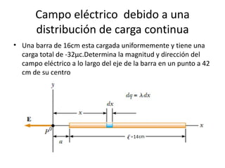
3. Campo eléctrico debido a una
distribución de carga continua
• Una barra de 16cm esta cargada uniformemente y tiene una
carga total de -32µc.Determina la magnitud y dirección del
campo eléctrico a lo largo del eje de la barra en un punto a 42
cm de su centro

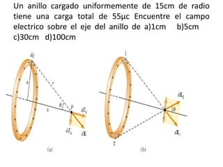
4. Un anillo cargado uniformemente de 15cm de radio
tiene una carga total de 55µc Encuentre el campo
electrico sobre el eje del anillo de a)1cm b)5cm
c)30cm d)100cm

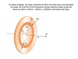
5. Un disco cargado de modo uniforme de 25cm de radio tiene una densidad
de carga de 5.6x10-3 C/m2.Calcule el campo electrico sobre el eje del
disco en a)5cm, b)10cm c)50cm y d)200cm del Centro del disco

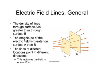
6. Electric Field Lines, General
• The density of lines
through surface A is
greater than through
surface B
• The magnitude of the
electric field is greater on
surface A than B
• The lines at different
locations point in different
directions
– This indicates the field is
non-uniform

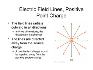
7. Electric Field Lines, Positive
Point Charge
• The field lines radiate
outward in all directions
– In three dimensions, the
distribution is spherical
• The lines are directed
away from the source
charge
– A positive test charge would
be repelled away from the
positive source charge

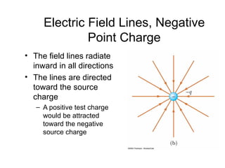
8. Electric Field Lines, Negative
Point Charge
• The field lines radiate
inward in all directions
• The lines are directed
toward the source
charge
– A positive test charge
would be attracted
toward the negative
source charge

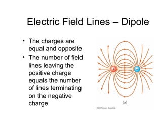
9. Electric Field Lines – Dipole
• The charges are
equal and opposite
• The number of field
lines leaving the
positive charge
equals the number
of lines terminating
on the negative
charge

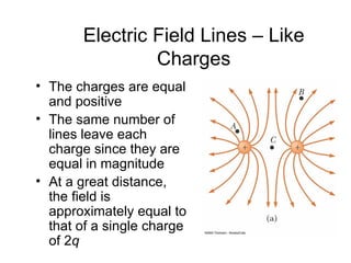
10. Electric Field Lines – Like
Charges
• The charges are equal
and positive
• The same number of
lines leave each
charge since they are
equal in magnitude
• At a great distance,
the field is
approximately equal to
that of a single charge
of 2q

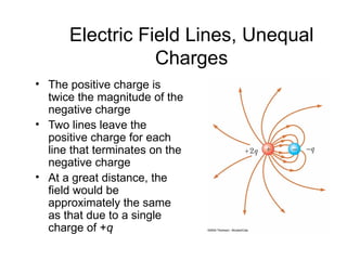
11. Electric Field Lines, Unequal
Charges
• The positive charge is
twice the magnitude of the
negative charge
• Two lines leave the
positive charge for each
line that terminates on the
negative charge
• At a great distance, the
field would be
approximately the same
as that due to a single
charge of +q

12. Motion of Particles, cont
• Fe = qE = ma
• If E is uniform, then a is constant
• If the particle has a positive charge, its
acceleration is in the direction of the field
• If the particle has a negative charge, its
acceleration is in the direction opposite the
electric field
• Since the acceleration is constant, the kinematic
equations can be used

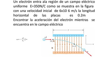
13. Un electrón entra ala región de un campo eléctrico
uniforme E=350N/C como se muestra en la figura
con una velocidad inicial de 6x10 6 m/s la longitud
horizontal de las placas es 0.2m
Encontrar la aceleración del electrón mientras se
encuentra en le campo eléctrico

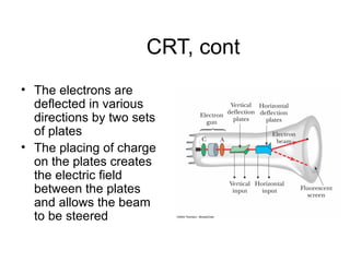
14. CRT, cont
• The electrons are
deflected in various
directions by two sets
of plates
• The placing of charge
on the plates creates
the electric field
between the plates
and allows the beam
to be steered

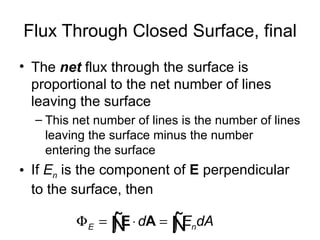
15. Flux Through Closed Surface, final
• The net flux through the surface is
proportional to the net number of lines
leaving the surface
– This net number of lines is the number of lines
leaving the surface minus the number
entering the surface
• If En is the component of E perpendicular
to the surface, then
Φ E = Ñ ⋅ dA = Ñ ndA
∫E ∫E

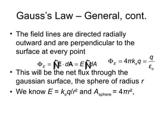
16. Gauss’s Law – General, cont.
• The field lines are directed radially
outward and are perpendicular to the
surface at every point
q
Φ E = Ñ ⋅ dA = E Ñ Φ E = 4πkeq =
∫E ∫ dA εo
• This will be the net flux through the
gaussian surface, the sphere of radius r
• We know E = keq/r2 and Asphere = 4πr2,

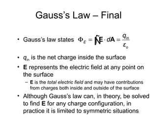
17. Gauss’s Law – Final
qin
• Gauss’s law states Φ E = Ñ ⋅ dA =
∫E εo
• qin is the net charge inside the surface
• E represents the electric field at any point on
the surface
– E is the total electric field and may have contributions
from charges both inside and outside of the surface
• Although Gauss’s law can, in theory, be solved
to find E for any charge configuration, in
practice it is limited to symmetric situations

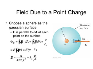
18. Field Due to a Point Charge
• Choose a sphere as the
gaussian surface
– E is parallel to dA at each
point on the surface
q
Φ E = Ñ ⋅ dA = Ñ
∫E ∫ EdA = εo
= E Ñ = Eπr
∫ dA (4
2
)
q q
E= 2
= ke 2
4πεo r r

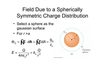
19. Field Due to a Spherically
Symmetric Charge Distribution
• Select a sphere as the
gaussian surface
• For r >a
qin
Φ E = Ñ ⋅ dA = Ñ
∫E ∫ EdA = εo
Q Q
E= 2
= ke 2
4πεo r r

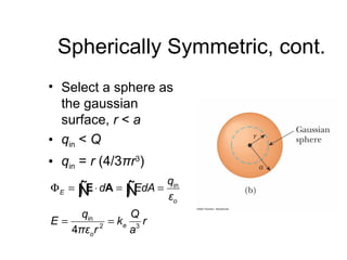
20. Spherically Symmetric, cont.
• Select a sphere as
the gaussian
surface, r < a
• qin < Q
• qin = r (4/3πr3)
qin
Φ E = Ñ ⋅ dA = Ñ
∫E ∫ EdA = εo
qin Q
E= 2
= ke 3 r
4πεo r a

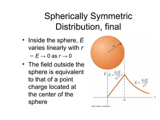
21. Spherically Symmetric
Distribution, final
• Inside the sphere, E
varies linearly with r
– E → 0 as r → 0
• The field outside the
sphere is equivalent
to that of a point
charge located at
the center of the
sphere

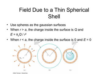
22. Field Due to a Thin Spherical
Shell
• Use spheres as the gaussian surfaces
• When r > a, the charge inside the surface is Q and
E = keQ / r2
• When r < a, the charge inside the surface is 0 and E = 0

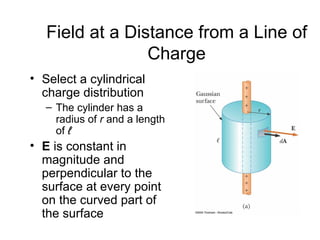
23. Field at a Distance from a Line of
Charge
• Select a cylindrical
charge distribution
– The cylinder has a
radius of r and a length
of ℓ
• E is constant in
magnitude and
perpendicular to the
surface at every point
on the curved part of
the surface

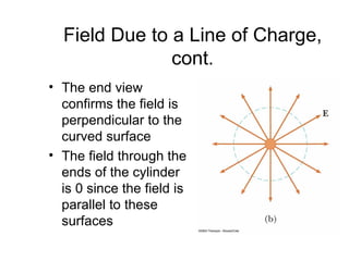
24. Field Due to a Line of Charge,
cont.
• The end view
confirms the field is
perpendicular to the
curved surface
• The field through the
ends of the cylinder
is 0 since the field is
parallel to these
surfaces

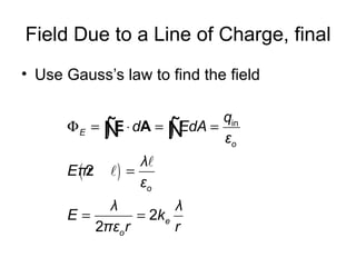
25. Field Due to a Line of Charge, final
• Use Gauss’s law to find the field
qin
Φ E = Ñ ⋅ dA = Ñ
∫E ∫ EdA = εo
λl
(2
Eπr l) =
εo
λ λ
E= = 2ke
2πεo r r

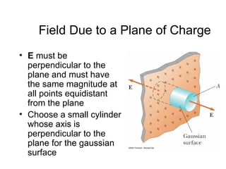
26. Field Due to a Plane of Charge
• E must be
perpendicular to the
plane and must have
the same magnitude at
all points equidistant
from the plane
• Choose a small cylinder
whose axis is
perpendicular to the
plane for the gaussian
surface

27. Field Due to a Plane of Charge,
cont
• E is parallel to the curved surface and
there is no contribution to the surface area
from this curved part of the cylinder
• The flux through each end of the cylinder
is EA and so the total flux is 2EA

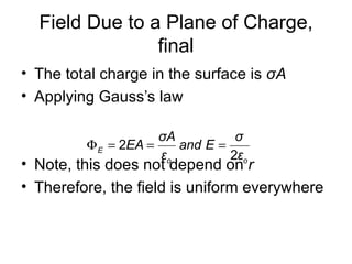
28. Field Due to a Plane of Charge,
final
• The total charge in the surface is σA
• Applying Gauss’s law
σA σ
Φ E = 2EA = and E =
εo 2εo
• Note, this does not depend on r
• Therefore, the field is uniform everywhere

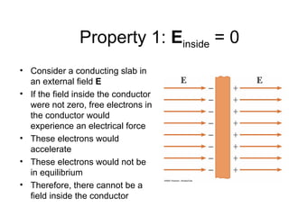
29. Property 1: Einside = 0
• Consider a conducting slab in
an external field E
• If the field inside the conductor
were not zero, free electrons in
the conductor would
experience an electrical force
• These electrons would
accelerate
• These electrons would not be
in equilibrium
• Therefore, there cannot be a
field inside the conductor

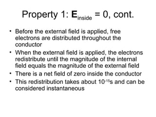
30. Property 1: Einside = 0, cont.
• Before the external field is applied, free
electrons are distributed throughout the
conductor
• When the external field is applied, the electrons
redistribute until the magnitude of the internal
field equals the magnitude of the external field
• There is a net field of zero inside the conductor
• This redistribution takes about 10-15s and can be
considered instantaneous

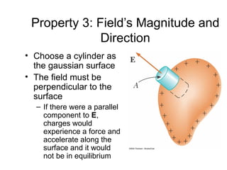
31. Property 3: Field’s Magnitude and
Direction
• Choose a cylinder as
the gaussian surface
• The field must be
perpendicular to the
surface
– If there were a parallel
component to E,
charges would
experience a force and
accelerate along the
surface and it would
not be in equilibrium

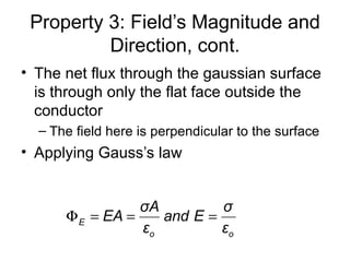
32. Property 3: Field’s Magnitude and
Direction, cont.
• The net flux through the gaussian surface
is through only the flat face outside the
conductor
– The field here is perpendicular to the surface
• Applying Gauss’s law
σA σ
Φ E = EA = and E =
εo εo

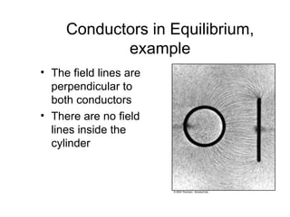
33. Conductors in Equilibrium,
example
• The field lines are
perpendicular to
both conductors
• There are no field
lines inside the
cylinder

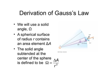
34. Derivation of Gauss’s Law
• We will use a solid
angle, Ω
• A spherical surface
of radius r contains
an area element ΔA
• The solid angle
subtended at the
center of the sphere
∆A
is defined to be Ω = 2
r

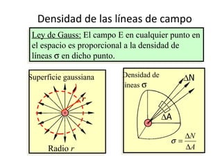
35. Densidad de las líneas de campo
Ley de Gauss: El campo E en cualquier punto en
el espacio es proporcional a la densidad de
líneas σ en dicho punto.
Superficie gaussiana Densidad de ∆N
líneas σ
r
∆A
∆N
σ=
Radio r ∆A

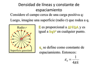
36. Densidad de líneas y constante de
espaciamiento
Considere el campo cerca de una carga positiva q:
Luego, imagine una superficie (radio r) que rodea a q.
Radio r E es proporcional a ∆N/∆A y es
igual a kq/r2 en cualquier punto.
r
∆N kq
∝ E; =E
∆A r 2
εο se define como constante de
Superficie gaussiana
espaciamiento. Entonces:
∆N 1
= ε 0E Donde ε 0 es : ε0 =
∆A 4π k

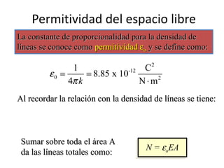
37. Permitividad del espacio libre
La constante de proporcionalidad para la densidad de
líneas se conoce como permitividad εο y se define como:
1 C2
ε0 = = 8.85 x 10-12
4π k N ⋅ m2
Al recordar la relación con la densidad de líneas se tiene:
∆N
= ε 0 E or ∆N = ε 0 E ∆A
∆A
Sumar sobre toda el área A
N = εoEA
da las líneas totales como:

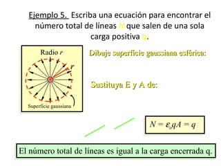
38. Ejemplo 5. Escriba una ecuación para encontrar el
número total de líneas N que salen de una sola
carga positiva q.
Radio r Dibuje superficie gaussiana esférica:
r ∆ N = ε 0 E∆ A y N = ε 0 EA
Sustituya E y A de:
kq q
E= 2 = ; A = 4π r 2
Superficie gaussiana r 4π r 2
 q 
N = ε 0 EA = ε 0  2 
(4π r 2 ) N = εoqA = q
 4π r 
El número total de líneas es igual a la carga encerrada q.

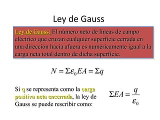
39. Ley de Gauss
Ley de Gauss: El número neto de líneas de campo
eléctrico que cruzan cualquier superficie cerrada en
una dirección hacia afuera es numéricamente igual a la
carga neta total dentro de dicha superficie.
N = Σε 0 EA = Σq
Si q se representa como la carga q
positiva neta encerrada, la ley de ΣEA =
Gauss se puede rescribir como: ε0

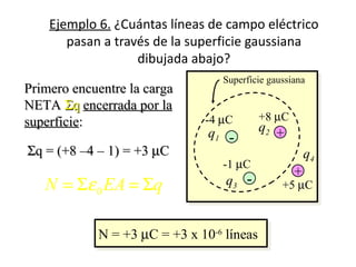
40. Ejemplo 6. ¿Cuántas líneas de campo eléctrico
pasan a través de la superficie gaussiana
dibujada abajo?
Superficie gaussiana
Primero encuentre la carga
NETA Σq encerrada por la
superficie: -4 µC +8 µC
q1 - q2 +
Σq = (+8 –4 – 1) = +3 µC q4
-1 µC
+
N = Σε 0 EA = Σq q3 - +5 µC
N = +3 µC = +3 x 10-6 líneas

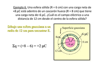
41. Ejemplo 6. Una esfera sólida (R = 6 cm) con una carga neta de
+8 µC está adentro de un cascarón hueco (R = 8 cm) que tiene
una carga neta de–6 µC. ¿Cuál es el campo eléctrico a una
distancia de 12 cm desde el centro de la esfera sólida?
Dibuje una esfera gaussiana a un Superficie gaussiana
radio de 12 cm para encontrar E.
- -6 µC
N = Σε 0 EA = Σq
8cm - -
- +8 µC -
6 cm
Σq = (+8 – 6) = +2 µC -
Σq 12 cm - -
ε 0 AE = qnet ; E =
ε0 A
Σq +2 x 10-6 C
E= =
ε 0 (4π r ) (8.85 x 10
2 -12 Nm 2
C 2 )(4π )(0.12 m)
2

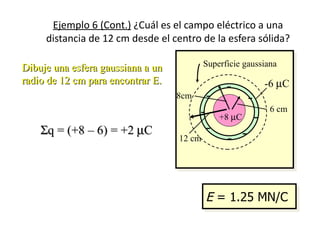
42. Ejemplo 6 (Cont.) ¿Cuál es el campo eléctrico a una
distancia de 12 cm desde el centro de la esfera sólida?
Superficie gaussiana
Dibuje una esfera gaussiana a un
radio de 12 cm para encontrar E. -6 µC
-
8cm - -
N = Σε 0 EA = Σq - 6 cm
+8 µC -
Σq = (+8 – 6) = +2 µC -
12 cm - -
Σq
ε 0 AE = qnet ; E =
ε0 A
+2 µ C
E= = 1.25 x 106 N C E = 1.25 MN/C
ε 0 (4π r 2 )

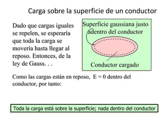
43. Carga sobre la superficie de un conductor
Dado que cargas iguales Superficie gaussiana justo
se repelen, se esperaría adentro del conductor
que toda la carga se
movería hasta llegar al
reposo. Entonces, de la
ley de Gauss. . . Conductor cargado
Como las cargas están en reposo, E = 0 dentro del
conductor, por tanto:
N = Σε 0 EA = Σq or 0 = Σq
Toda la carga está sobre la superficie; nada dentro del conductor

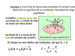
44. Ejemplo 7. Use la ley de Gauss para encontrar el campo E just
afuera de la superficie de un conductor. Densidad de carga
superficial: σ = q/A.
Considere q adentro de la caja.
E3 E1 E3
Las líneas de E a través de todas
las áreas son hacia afuera. A
+3 + + + + +3
Σε 0 AE = q +E E
E2 +
++ + + +
Las líneas de E a través de los
lados se cancelan por simetría. Densidad de carga superficial σ
El campo es cero dentro del conductor, así que E2 = 0
0 q σ
εoE1A + εoE2A = q E= =
ε0 A ε0

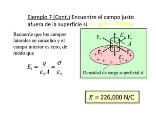
45. Ejemplo 7 (Cont.) Encuentre el campo justo
afuera de la superficie si σ = q/A = +2 C/m2.
Recuerde que los campos E1 E3
E3
laterales se cancelan y el
campo interior es cero, de A
+3 + + + + +3
modo que +E E
E2 +
++ + + +
q σ
E1 = =
ε0 A ε0 Densidad de carga superficial σ
+2 x 10-6 C/m 2
E= -12 Nm 2 E = 226,000 N/C
8.85 x 10 C2

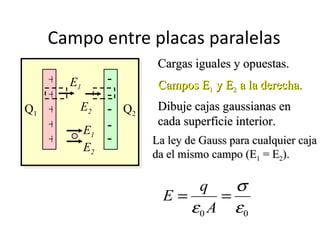
46. Campo entre placas paralelas
Cargas iguales y opuestas.
+ E1 - Campos E1 y E2 a la derecha.
+ -
Q1 + E2 - Q2 Dibuje cajas gaussianas en
+ - cada superficie interior.
E1
+ - La ley de Gauss para cualquier caja
E2
da el mismo campo (E1 = E2).
q σ
Σε 0 AE = Σq E= =
ε0 A ε0

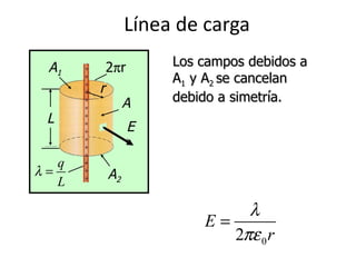
47. Línea de carga
A1 2πr Los campos debidos a
A1 y A2 se cancelan
r
A debido a simetría.
L Σε 0 AE = q
E
q
λ=
q EA = ; A = (2π r ) L
L
A2 ε0
q q λ
E= ; λ= E=
2πε 0 rL L 2πε 0 r

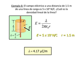
48. Ejemplo 8: El campo eléctrico a una distancia de 1.5 m
de una línea de carga es 5 x 104 N/C. ¿Cuál es la
densidad lineal de la línea?
r λ
E= λ = 2πε 0 rE
L E 2πε 0 r
q
λ= E = 5 x 104 N/C r = 1.5 m
L
λ = 2π (8.85 x 10 -12 C2
Nm 2
4
)(1.5 m)(5 x 10 N/C)
λ = 4.17 µC/m

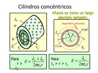
49. Cilindros concéntricos
Afuera es como un largo
alambre cargado:
λb ++
++++ Superficie gaussiana
a +++++
++++ -6 µC
+++ ra
++
b ++ λa rb
λa r r2 12 cm λb
1
Para λa + λb Para λa
E= E=
r> 2πε 0 r rb > r > ra 2πε 0 r
rb

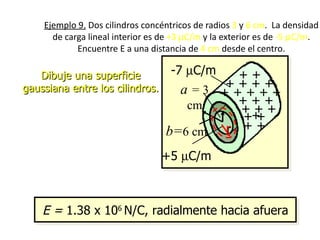
50. Ejemplo 9. Dos cilindros concéntricos de radios 3 y 6 cm. La densidad
de carga lineal interior es de +3 µC/m y la exterior es de -5 µC/m.
Encuentre E a una distancia de 4 cm desde el centro.
Dibuje una superficie -7 µC/m ++
gaussiana entre los cilindros. ++++
a=3 +++++
cm +++
λb +++
+++
E=
2πε 0 r b=6 cm r + +
+3µ C/m +5 µC/m
E=
2πε 0 (0.04 m)
E = 1.38 x 106 N/C, radialmente hacia afuera

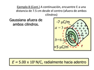
51. Ejemplo 8 (Cont.) A continuación, encuentre E a una
distancia de 7.5 cm desde el centro (afuera de ambos
cilindros)
Gaussiana afuera de
-7 µC/m ++
ambos cilindros. ++++
a = 3 cm + + + + +
λa + λb +++
E= +++
2πε 0 r +++
b=6 cm ++
(+3 − 5) µ C/m
E= +5 µC/m r
2πε 0 (0.075 m)
E = 5.00 x 105 N/C, radialmente hacia adentro

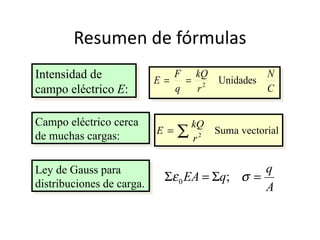
52. Resumen de fórmulas
Intensidad de E=
F kQ
= 2 Unidades
N
campo eléctrico E: q r C
Campo eléctrico cerca kQ
E =∑ 2 Suma vectorial
de muchas cargas: r
Ley de Gauss para q
Σε 0 EA = Σq; σ =
distribuciones de carga. A

53. CONCLUSIÓN: Capítulo 24
El campo eléctrico