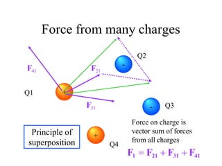
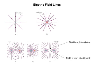
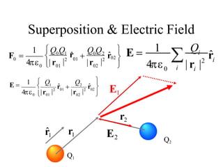
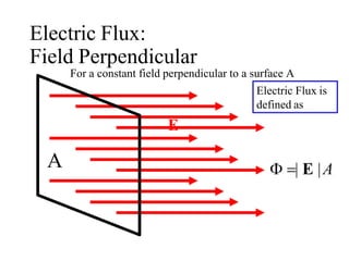
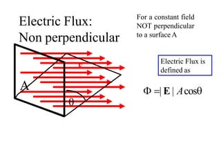
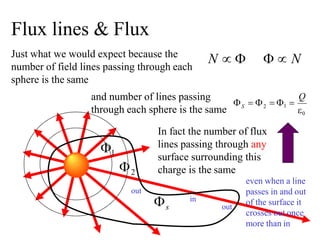
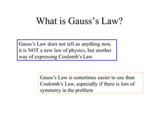
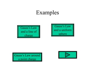
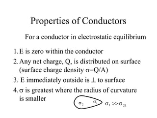
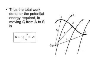
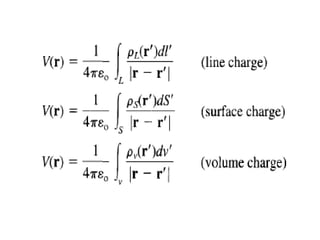
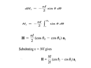
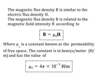
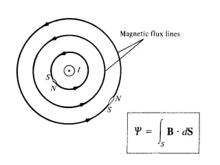
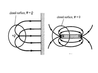
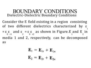
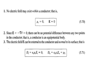
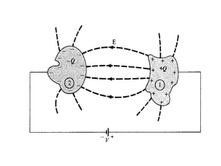
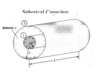
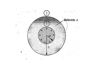
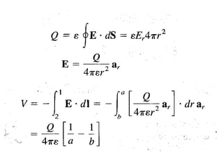
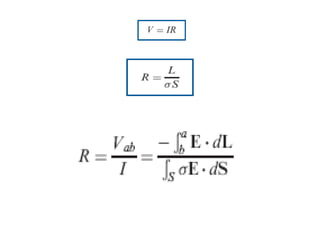
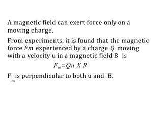
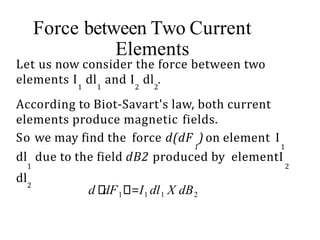
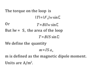
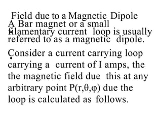
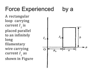
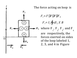
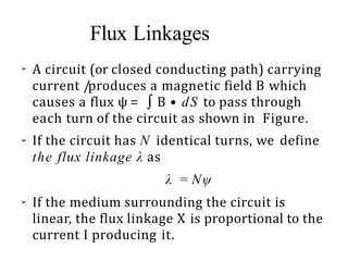
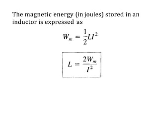
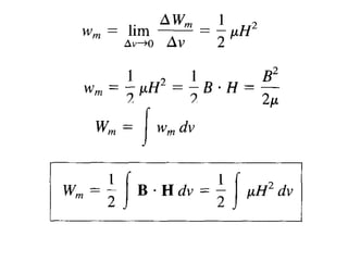
This document provides an introduction to the concept of electromagnetic fields. It begins by discussing electrostatics and defining electric fields as having their sources in electric charges. It then covers Coulomb's law, which describes the electric force between two charges, and Gauss's law, which relates the electric flux through a closed surface to the electric charge enclosed. The document explains electric field lines and flux, superposition of electric fields, and uses Gauss's law to analyze properties of conductors. Finally, it mentions that the next section will cover electric potential. The key information is that the document serves as an introduction to electromagnetic fields, covering fundamental concepts like Coulomb's and Gauss's laws.


![F4= I2
0
∮
= 0 a
d a X
I
0 1
0
2 a
a
F4=
− I1 I2
2
ln
0 a
0
az
(Parallel)
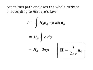
The Total Force
Fl =
I1 I2 b 1
0
[ −
1
0
2 a
] −a](https://image.slidesharecdn.com/emfppt0-231004183608-bfbdf42e/85/EMF-PPT_0-pdf-200-320.jpg)


![Human Reproduction [ Reproductive System ] Notes @irfanullah_mehar Irfanullah...](https://cdn.slidesharecdn.com/ss_thumbnails/humanreproductionreproductivesystemnotesirfanullahmeharirfanullahmeharjanantantra-260111172350-56e85778-thumbnail.jpg?width=640&height=640&fit=bounds)


