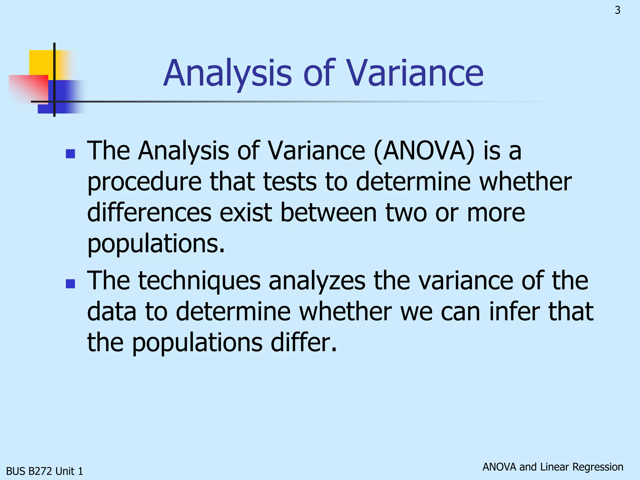
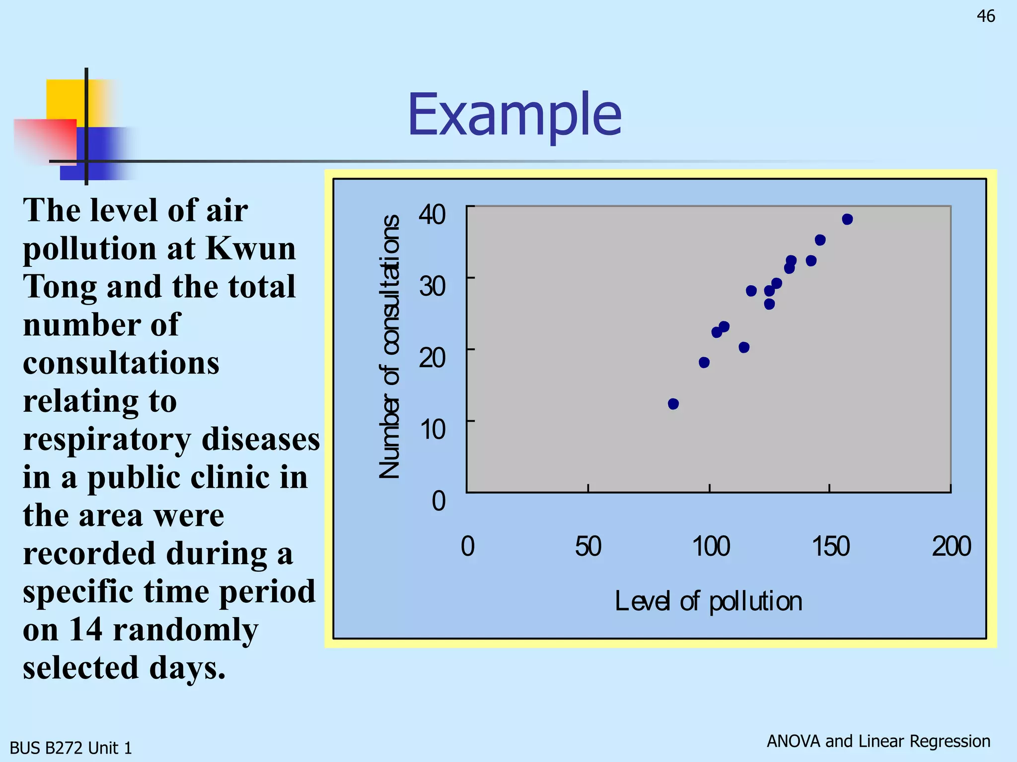
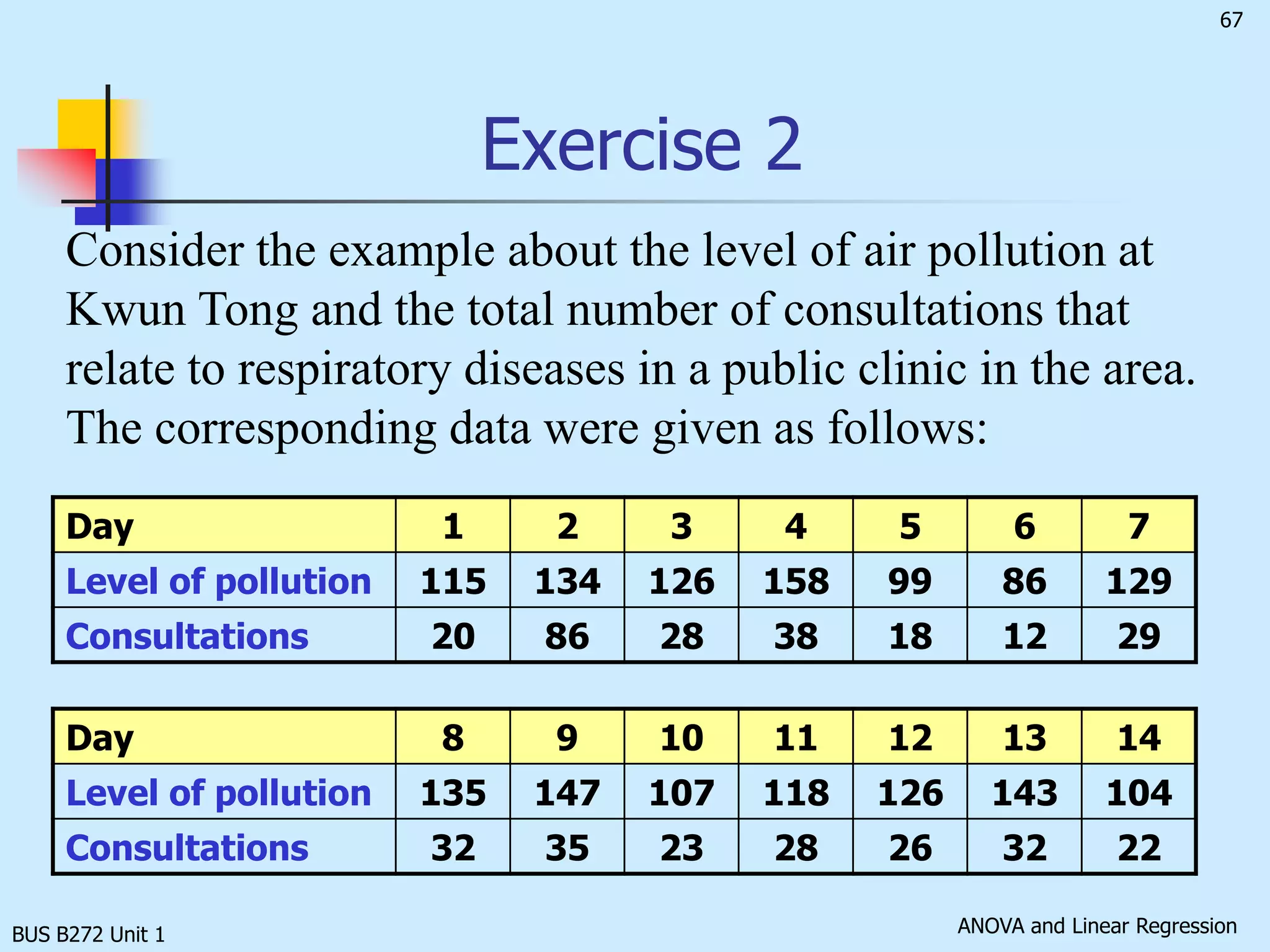
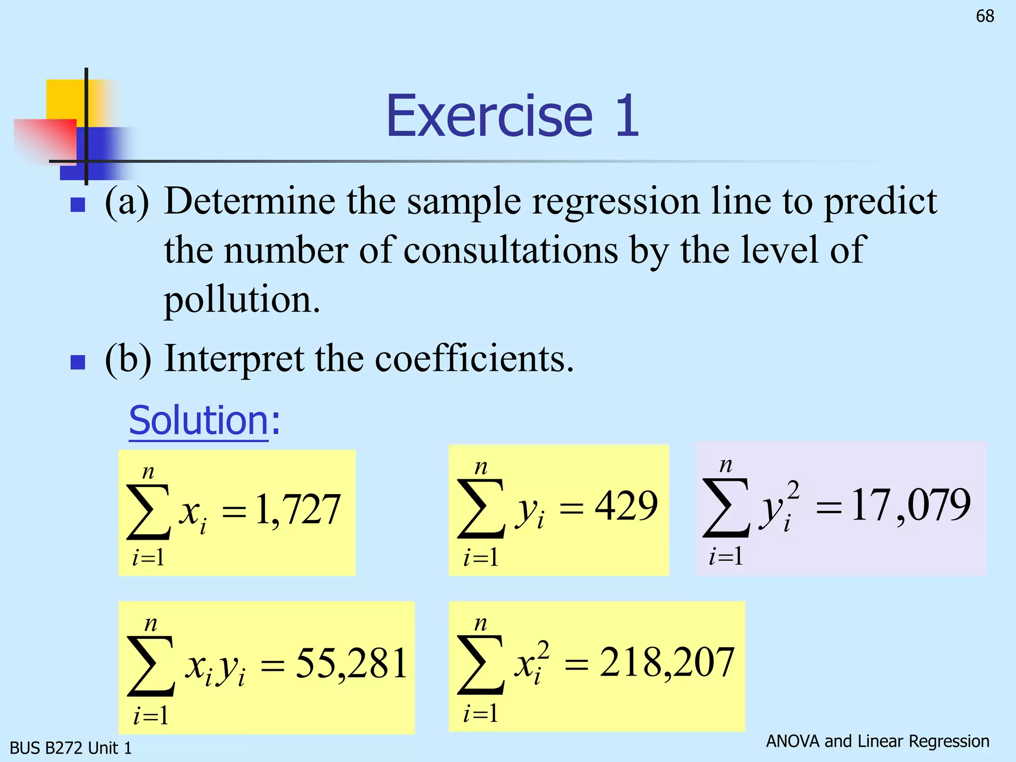
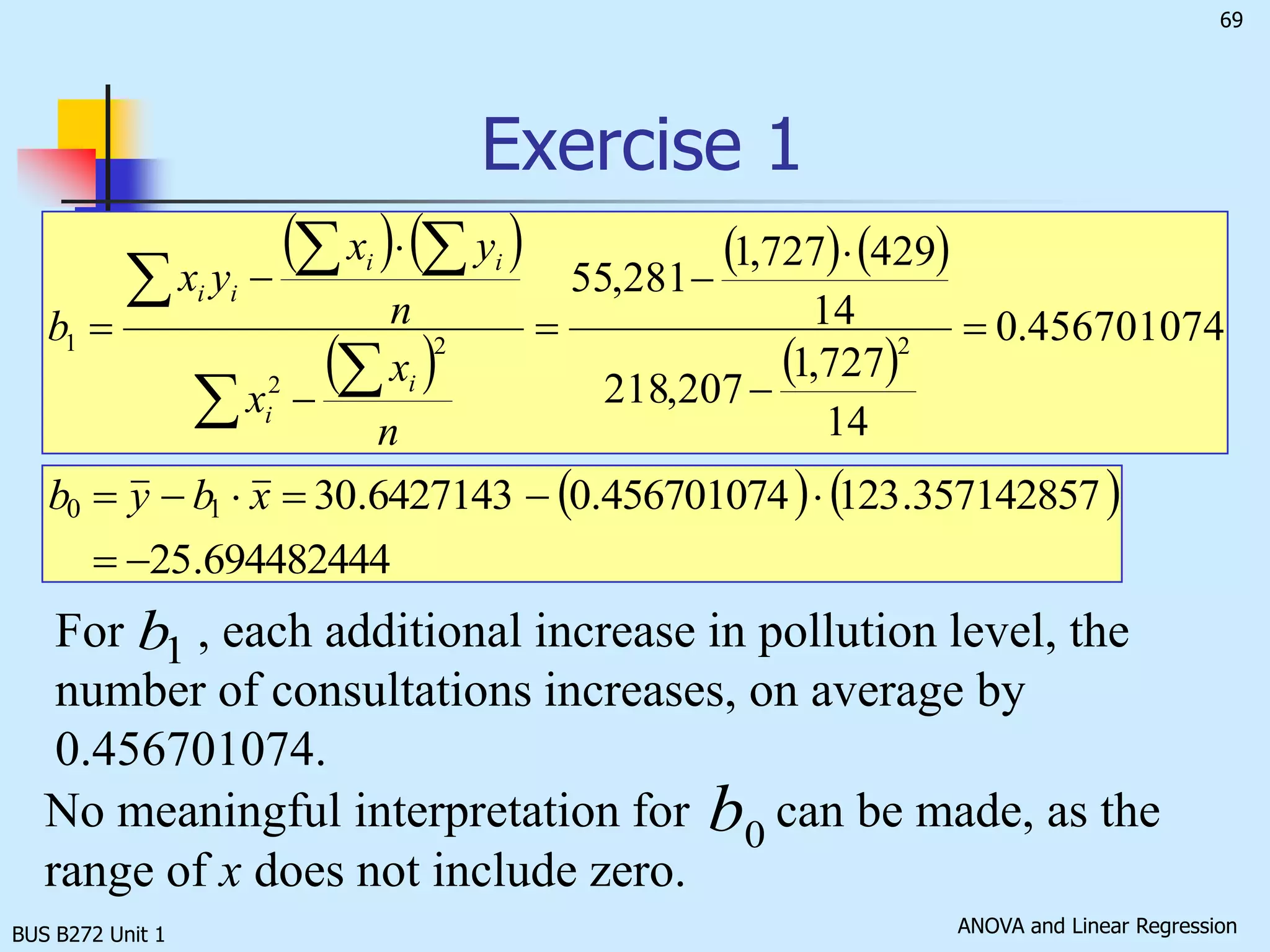
The document discusses analysis of variance (ANOVA) and linear regression. It provides an overview of ANOVA, including one-way ANOVA, its assumptions, hypotheses, and F-test. It also discusses linear regression, including determining the simple linear regression equation, assessing model fitness, correlation analysis, and assumptions of regression. As an example, it analyzes a study on the relationship between air pollution levels and respiratory disease consultations using these statistical techniques.

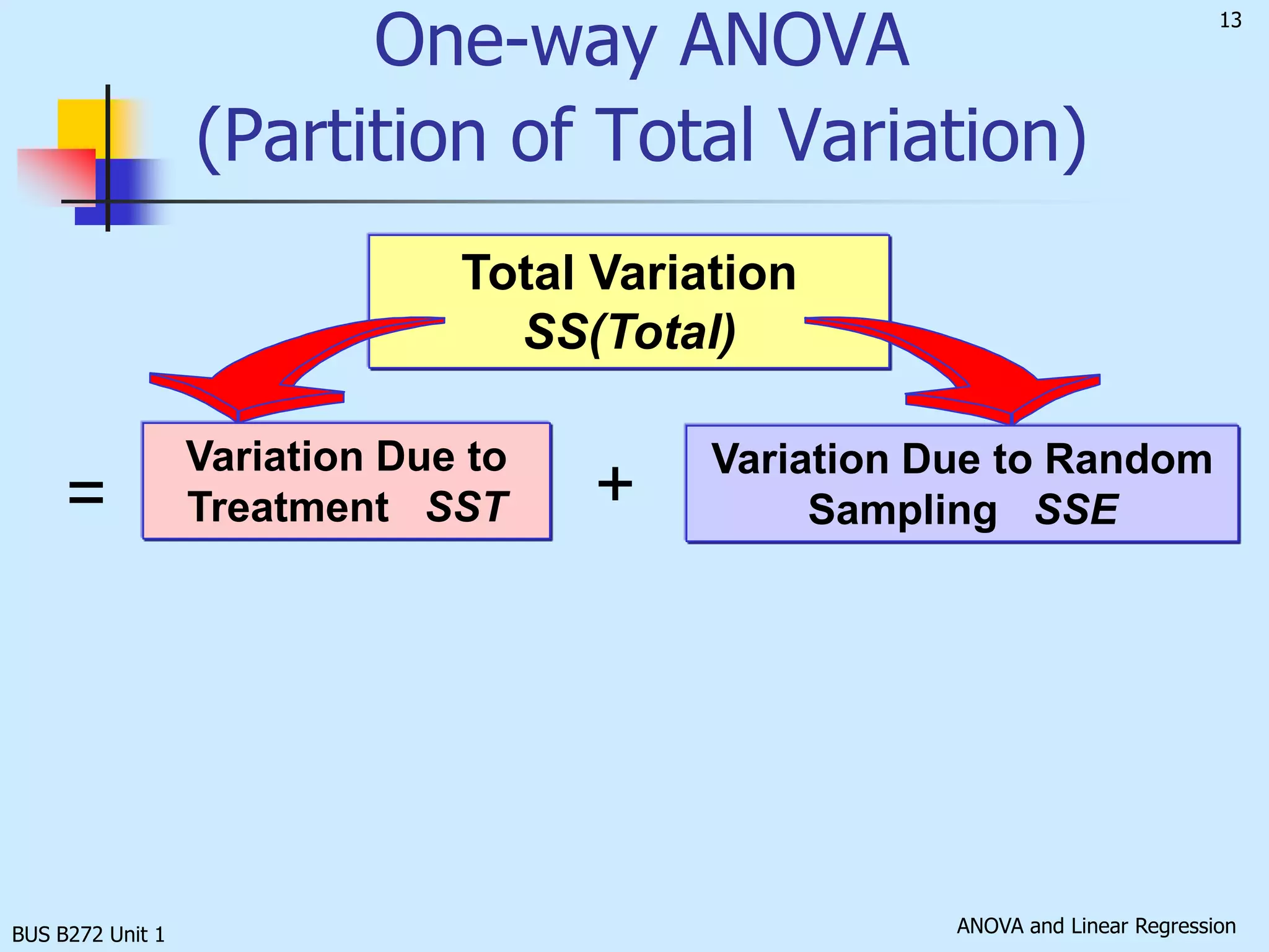


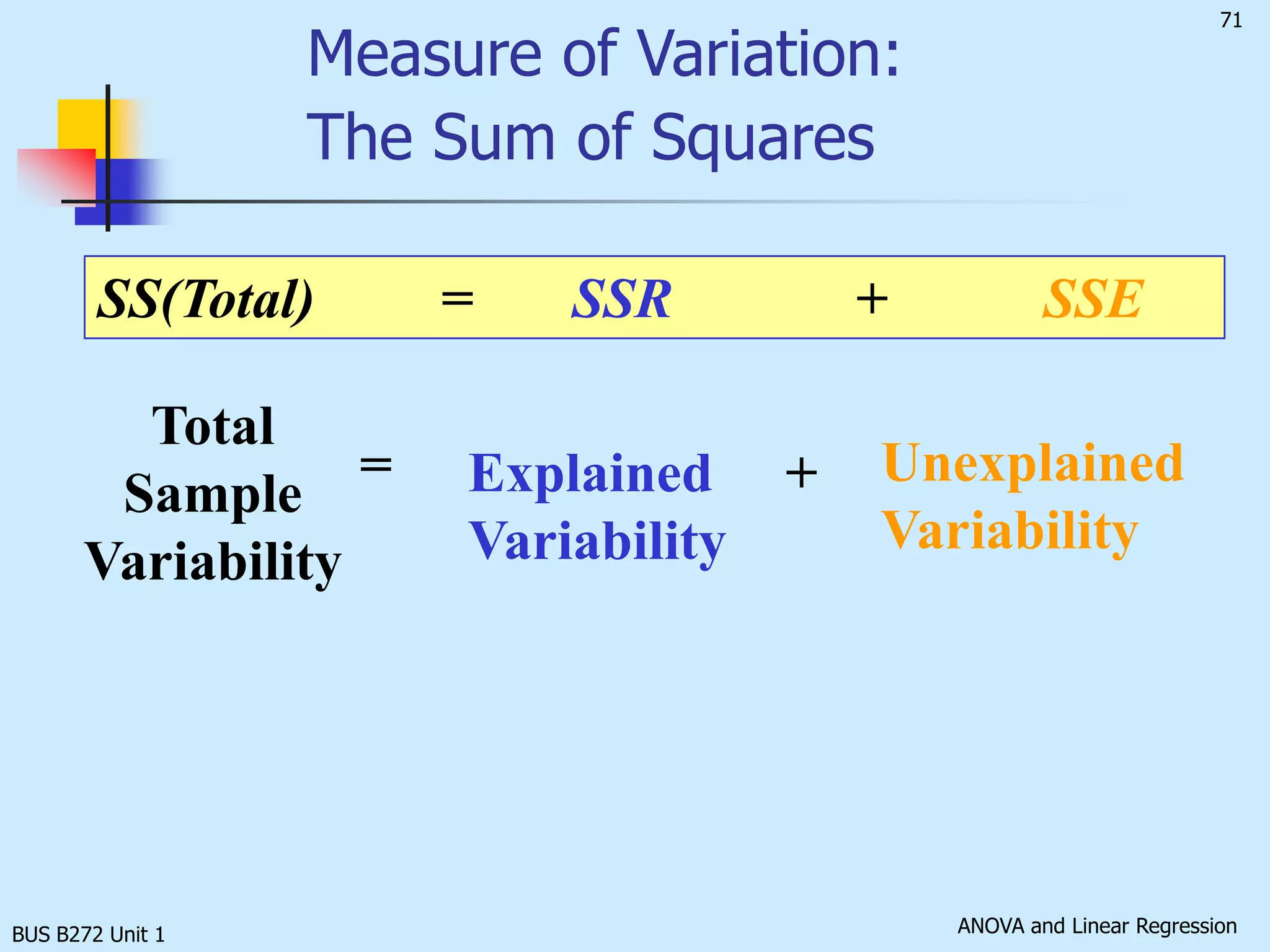


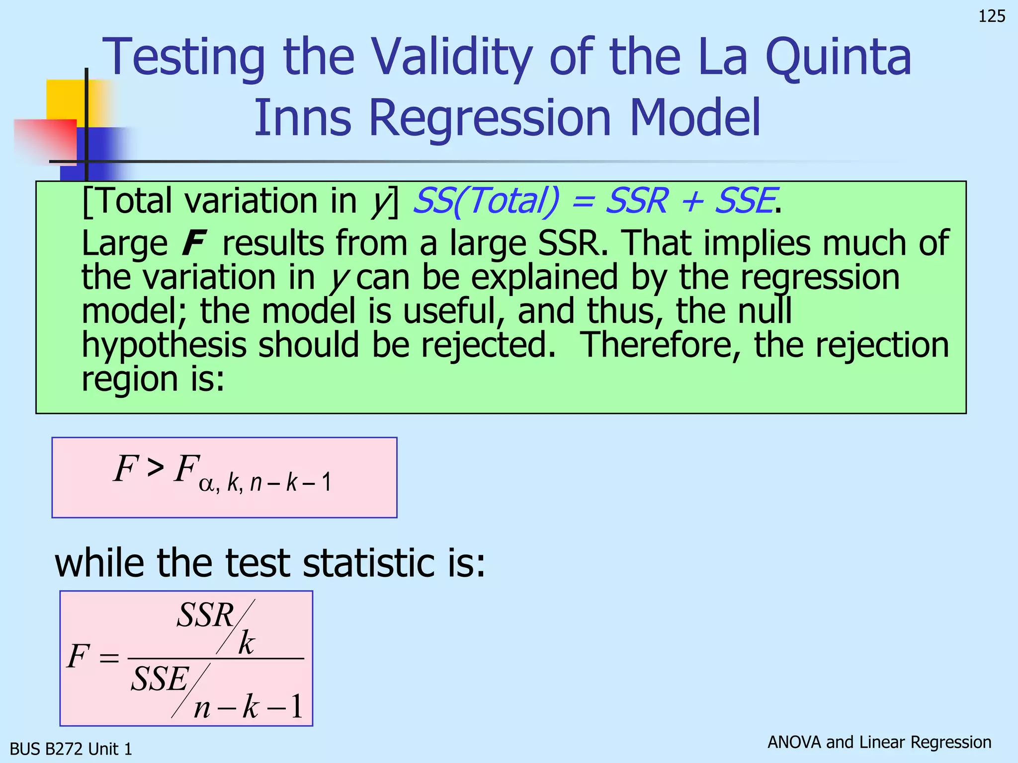
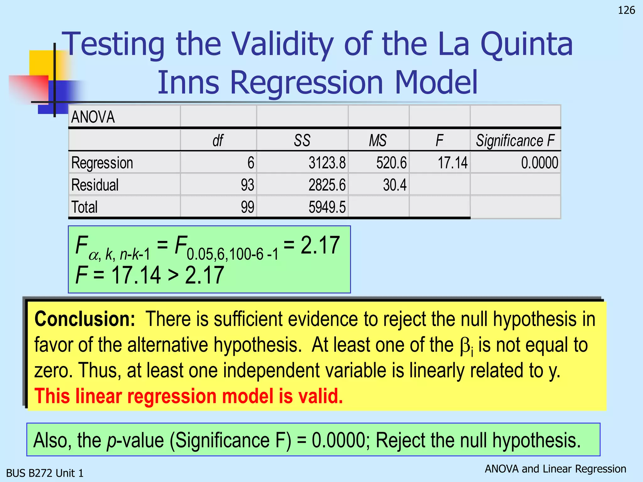
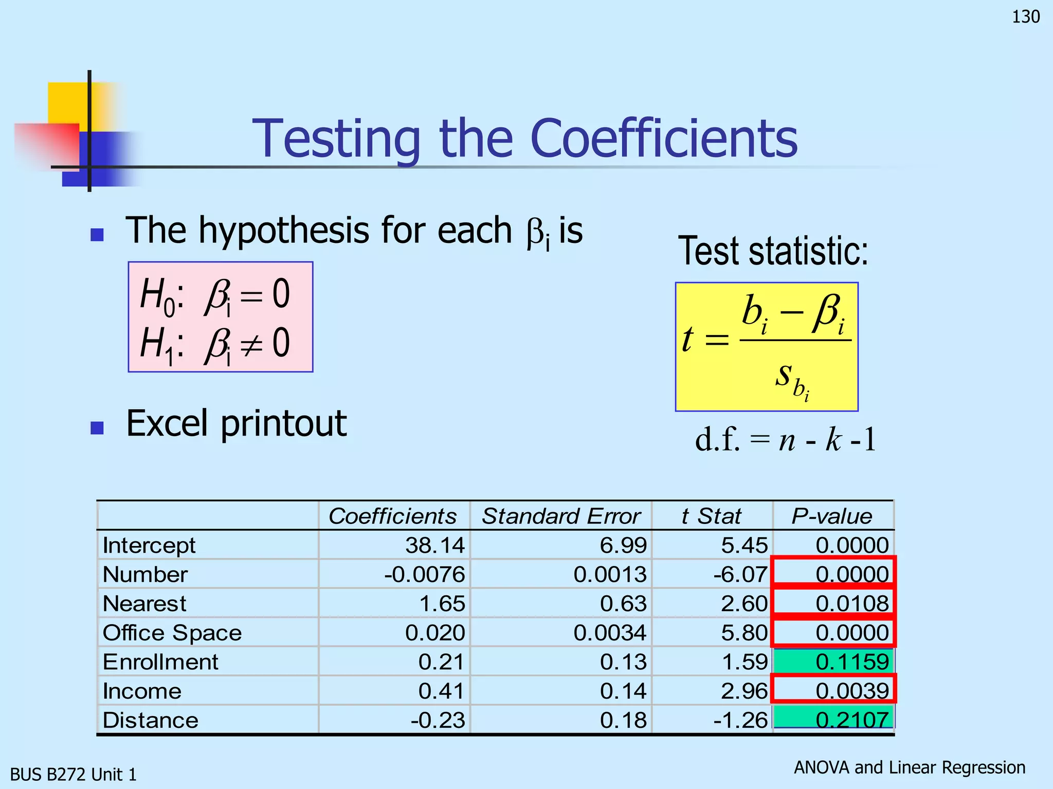
![BUS B272 Unit 1Testing the Validity of the La Quinta Inns Regression Model [Total variation in y] SS(Total) = SSR + SSE. Large F results from a large SSR. That implies much of the variation in y can be explained by the regression model; the model is useful, and thus, the null hypothesis should be rejected. Therefore, the rejection region is:F > Fa, k, n – k – 1while the test statistic is:](https://image.slidesharecdn.com/busb272funit1-110423015457-phpapp01/75/Bus-b272-f-unit-1-132-2048.jpg)