This document presents two stochastic inventory models (Models A and B) with randomly varying environments. Model A has a maximum demand size (M) that is greater than the maximum supply size (N) across environments. The state of the inventory system is represented by a continuous time Markov chain. Model A's infinitesimal generator matrix is partitioned into blocks to exhibit a matrix geometric structure. Stationary probabilities, expected values, and variances are derived for the number of demands waiting and inventory levels using the matrix geometric results.

1. IOSR Journal of Mathematics (IOSR-JM)
e-ISSN: 2278-5728, p-ISSN: 2319-765X. Volume 11, Issue 1 Ver. 1 (Jan - Feb. 2015), PP 75-82
www.iosrjournals.org
DOI: 10.9790/5728-11117582 www.iosrjournals.org 75 | Page
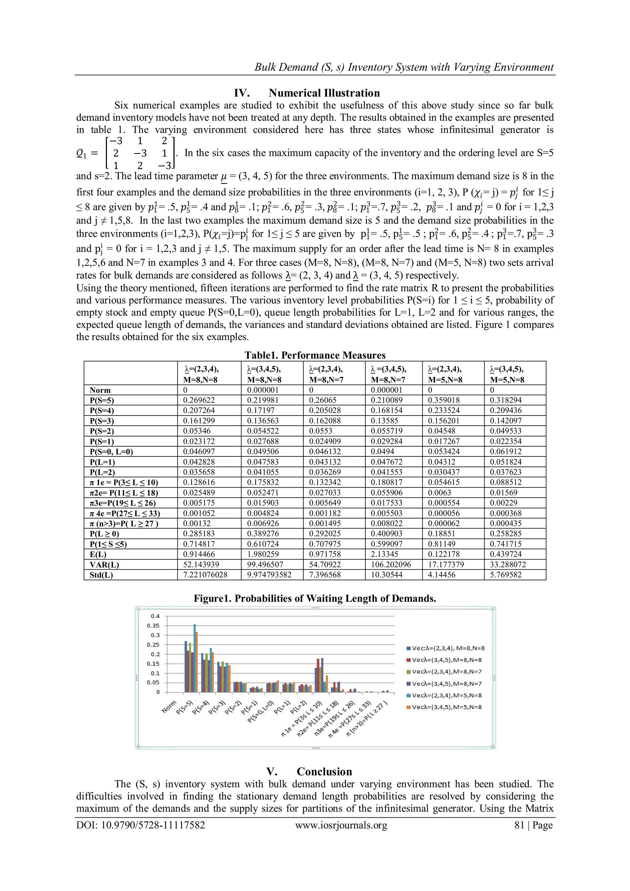
Bulk Demand (S, s) Inventory System with Varying
Environment
Sundar Viswanathan1
, Rama Ganesan2
, Ramshankar.R3
, Ramanarayanan.R4
1
Senior Testing Engineer, ANSYS Inc., 2600, ANSYS Drive, Canonsburg, PA 15317, USA
2
Independent Researcher B.Tech, Vellore Institute of Technology, Vellore, India
3
Independent Researcher MS9EC0, University of Massachusetts, Amherst, MA, USA
4
Professor of Mathematics, (Retired), Dr.RR & Dr.SR Technical University, Chennai.
Abstract: This paper studies two stochastic bulk demand (S, s) inventory models A and B with randomly
varying environment. In the models the maximum storing capacity of the inventory is S units and the order for
filling up the inventory is placed when the inventory level falls to s or below. Demands for random number of
units occur at a time and wait for supply forming a queue when the inventory has no stock. The inventory is
exposed to changes in the environment. Inter occurrence time between consecutive bulk demands has
exponential distribution and its parameter changes when the environment changes. Lead time for an order
realization has exponential distribution and its parameter also changes when the environment changes. When
an order is realized in the environment i, for 1 ≤ i ≤ k, the inventory is filled up if no demand is waiting or if the
number n of demands waiting is such that 0 ≤ n ≤ 𝑁𝑖-S where 𝑁𝑖is the maximum number of units supplied in the
environment i for an order. If n is such that with 𝑁𝑖-S < n < 𝑁𝑖 all the n demands are cleared and 𝑁𝑖-n units
become stocks for the inventory if 𝑁𝑖-n ≤ S and if 𝑁𝑖-n >S the inventory is filled up and the units in excess after
filling up the inventory are returned. If n ≥ 𝑁𝑖 demands are waiting, 𝑁𝑖 demands are cleared reducing the
demand level to n-𝑁𝑖. In model A, 𝑚𝑎𝑥𝑖 𝑀𝑖 >𝑚𝑎𝑥𝑖 𝑁𝑖 where 𝑀𝑖 is the maximum demand size in the environment
i for1≤ i ≤ k. In model B the maximum demand size in all environments is less than maximum supply size in all
environments. Matrix partitioning method is used to study the models. The stationary probabilities of demand
length, its expected values, its variances and probabilities of empty levels are derived for the two models using
the iterated rate matrix. Numerical examples are presented for illustration.
Keywords: Block Circulant Matrix, Block partitioning methods, Bulk Demands, Lead time, Matrix Geometric
Methods.
I. Introduction
In this paper two bulk demand (S, s) inventory systems with varying environment are treated using
matrix geometric methods. Thangaraj and Ramanarayanan [1] have studied two ordering level and unit demand
inventory systems using integral equations. Jacob and Ramanarayanan [2] have treated (S, s) inventory systems
with server vacations. Ayyappan, Subramanian and Gopal Sekar [3] have analyzed retrial system using matrix
geometric methods. Bini, Latouche and Meini [4] have studied numerical methods for Markov chains.
Chakravarthy and Neuts [5] have discussed in depth a multi-server waiting model. Gaver, Jacobs and Latouche
[6] have treated birth and death models with random environment. Latouche and Ramaswami [7] have studied
Analytic methods. For matrix geometric methods and models one may refer Neuts [8]. Rama Ganesan,
Ramshankar and Ramanarayanan [9] have analyzed M/M/1 bulk queues under varying environment. Fatigue
failure models using Matrix geometric methods have been analyzed by Sundar [10]. The models considered in
this paper are general compared to existing inventory models. Here at each environment in a demand epoch,
random numbers of units are demanded and the maximum number of units demanded may be different in the
various environments. When there is no stock in the inventory, after the lead time, realized orders can clear in
each environment various number of waiting demands. Usually bulk arrival models have M/G/1 upper-
Heisenberg block matrix structure with zeros below the first sub diagonal. The decomposition of a Toeplitz sub
matrix of the infinitesimal generator is required to find the stationary probability vector. Matrix geometric
structures have not been noted as mentioned by William J. Stewart [11] and even in such models the recurrence
relation method to find the stationary probabilities is stopped at certain level in most general cases indicating
limitations of such approach. Rama Ganesan and Ramanarayanan [12] have presented a special case where a
generating function has been noticed in such a situation. But in this paper the partitioning of the matrix with
blocks of size, which is the maximum of the maximum number of demands and the maximum of the order
supply sizes in all the environments, exhibits the matrix geometric structure for the varying environment (S, s)
inventory system. This shows (S, s) inventory systems of M/M/1 types with bulk arrivals of demands no matter
how big the demand size is in number at each arrival epoch provided it is bounded above by a maximum and the

2. Bulk Demand (S, s) Inventory System with Varying Environment
DOI: 10.9790/5728-11117582 www.iosrjournals.org 76 | Page
supply for orders after the lead time no matter how big the supply size is in number provided it is bounded
above by a maximum, have matrix geometric solutions.
Two models (A) and (B) of bulk demand (S, s) inventory systems with k varying environments and
infinite storage spaces for demands are studied here using the block partitioning method and matrix geometric
results are obtained. In the models considered here, the maximum demand sizes and the maximum order supply
sizes are different for different environments. Model (A) presents the case when M, the maximum of all the
maximum demand sizes in all the environments is bigger than N, the maximum of order supply sizes in all the
environments. In Model (B), its dual case, N is bigger than M, is treated. In general in waiting line models, the
state space of the system has the first co-ordinate indicating the number of customers in the system but here the
demands in the system are grouped and considered as members of M sized blocks of demands (when M >N) or
N sized blocks of demands (when N > M) for finding the rate matrix. Using the maximum of the bulk demand
sizes or the maximum of the order supply sizes with grouping of the demands as members of the blocks for the
partitioning of the infinitesimal generator is a new approach in this area. The matrices appearing as the basic
system generators in these two models due to block partitions are seen as block circulants. The stationary
probability of the number of demands waiting for service, the expectation, the variance and the probability of
various levels of the inventory are derived for these models. Numerical cases are presented to illustrate their
applications. The paper is organized in the following manner. In section II the (S, s) inventory system with bulk
demand and order clearance after the lead time is studied for randomly varying environment in which
maximum M is greater than maximum N. Section III treats the situation in which the maximum M is less than
the maximum N. In section IV numerical cases are presented.
.
II. Model (A). Maximum Demand Size M is Greater Than The Maximum Supply Size N
2.1Assumptions for M > N.
i) There are k environments. The environment changes as per changes in a continuous time Markov chain
with infinitesimal generator 𝒬1 of order k.
ii) Demands arrive for multiple numbers of units at demand epochs. The time between consecutive demand
epochs has exponential distribution with parameterλi, in the environment i for 1 ≤ i ≤ k. At each demand
epoch in the environment i, χi units are demanded with probability given by P (χi= j) = pj
i
for 1 ≤ j ≤ Mi
where Mi is the maximum number of units of demand and pj
iMi
j=1 =1 for 1 ≤ i ≤ k.
iii) The maximum capacity of the inventory to store units is S. Whenever the inventory level falls to s or below,
orders are made for the supply of units for the inventory. Arriving demands are served till the inventory
level falls to 0 after which the demands wait for order realization. During the lead time of an order, another
order cannot be made. After the realization of an order if the inventory level becomes s or below s or the
inventory is still empty with or without waiting demands, then the next order is made. When an order is
realized in the environment i, for 1 ≤ i ≤ k the inventory is supplied with Ni ≥ S units. When the inventory
level is in between 0 and s, the inventory is filled up and units which are in excess are returned
immediately. When n demands are waiting for 0 ≤ n ≤ Ni-S at the order realization epoch, n waiting
demands are cleared, the inventory is filled up and units in excess are immediately returned. When the
waiting number of demands n at the order realization epoch is such that Ni-S < n < Ni all the n demands are
cleared and Ni-n units become stocks for the inventory if Ni-n ≤ S and if Ni-n > S the inventory is filled up
and the units in excess are returned. If n ≥ Ni demands are waiting when an order is realized, Ni demands
are cleared reducing the waiting demand level to n-Ni. The lead time distribution of an order has
exponential distribution with parameter μi in the environment i for1 ≤ i ≤ k.
iv) iv)When the environment changes from i to j, the parameter λi of inter occurrence time of bulk demands
and the parameter of the lead time of an order μi change to λj and μj respectively and the maximum
demand size Mi and the order realization size Ni change to Mj and Nj respectively for1 ≤ i, j ≤ k.
v) The maximum of the maximum of demand sizes M = max1 ≤i ≤k Mi is greater than the maximum of the
order realization sizes N =max1 ≤i ≤k Ni.
2.2 Analysis
The state of the system of the continuous time Markov chain X (t) under consideration is presented as
follows.
X (t) = {(n, j, i): for 0 ≤ j ≤ M-1; 1 ≤ i ≤ k and n ≥ 0} (1)
The chain is in the state (0, j, i) when the S – j units are in the inventory for 0 ≤ j ≤ S and the
environment is in state is i for 1 ≤ i ≤ k. The chain is in the state (0, j, i) when j-S demands are waiting for S+1≤
j ≤ M-1 and the environment state is i, for1 ≤ i ≤ k. The chain is in the state (n, j, i) when the number of demands
waiting for units is n M + j - S, for 0 ≤ j ≤ M-1, 1 ≤ n < ∞ and the environment state is i for 1 ≤ i ≤ k. When the
number of demands in the system is r ≥ 1, then r is identified with (n, j) where r + S on division by M gives n as

3. Bulk Demand (S, s) Inventory System with Varying Environment
DOI: 10.9790/5728-11117582 www.iosrjournals.org 77 | Page
the quotient and j as the remainder. When the inventory level is r, for 0 ≤ r ≤ S without any waiting demand at
level 0 then r is identified with (0, j) where j= S – r, for 0 ≤ j ≤ S.
The chain X (t) describing model has the infinitesimal generator QA of infinite order which can be presented in
block partitioned form given below.
QA =
B1 A0 0 0 . . . ⋯
A2 A1 A0 0 . . . ⋯
0 A2 A1 A0 0 . . ⋯
0 0 A2 A1 A0 0 . ⋯
0 0 0 A2 A1 A0 0 ⋯
⋮ ⋮ ⋮ ⋮ ⋱ ⋱ ⋱ ⋱
(2)
In (2) the states of the matrix are listed lexicographically as 0, 1, 2, 3, … . n, …. Here the vector n is of type 1 x
k M and n = ((n, 0, 1), (n, 0, 2) …(n, 0, k), (n, 1, 1), (n, 1, 2),…(n, 1, k),…(n, M-1, 1), (n, M-1, 2)…
(n, M-1, k) for n ≥ 0.
The matrices B1and A1 have negative diagonal elements, they are of order Mk and their off diagonal
elements are non- negative. The matrices A0, andA2 have nonnegative elements and are of order Mk and they
are given below. Let the following be diagonal matrices of order k
Λj=diag (λ1pj
1
, λ2pj
2
, … . , λk pj
k
) for 1 ≤ j ≤ M; (3)
Ujis 0 matrix of order k for 1 ≤ j ≤ N except for j = Ni for 1 ≤ i ≤ k and S ≤ Ni ≤ N where UNi
is a
matrix of order k with only one non zero element (UNi
)i,i = μi for 1 ≤ i ≤ k and its other elements are 0. (4)
Vj = Ui
N
i=j+1 for 1 ≤ j ≤ N − 1 Λ = diag (λ1, λ2, … . , λk ); (5)
and U = diag μ1, μ2, … . , μk = Ui
N
i=1 . (6)
Let 𝒬1
′
= 𝒬1 − Λ − U. (7)
Here 𝒬1 is the infinitesimal generator of the Markov chain of the environment.
A0 =
ΛM 0 ⋯ 0 0 0
ΛM−1 ΛM ⋯ 0 0 0
ΛM−2 ΛM−1 ⋯ 0 0 0
ΛM−3 ΛM−2 ⋱ 0 0 0
⋮ ⋮ ⋱ ⋱ ⋮ ⋮
Λ3 Λ4 ⋯ ΛM 0 0
Λ2 Λ3 ⋯ ΛM−1 ΛM 0
Λ1 Λ2 ⋯ ΛM−2 ΛM−1 ΛM
(8) A2 =
0 ⋯ 0 UN UN−1 ⋯ U2 U1
0 ⋯ 0 0 UN ⋯ U3 U2
⋮ ⋮ ⋮ ⋮ ⋮ ⋱ ⋮ ⋮
0 ⋯ 0 0 0 ⋯ UN UN−1
0 ⋯ 0 0 0 ⋯ 0 UN
0 ⋯ 0 0 0 ⋯ 0 0
⋮ ⋮ ⋮ ⋮ ⋮ ⋮ ⋮ ⋮
0 ⋯ 0 0 0 ⋯ 0 0
(9)
A1 =
𝒬1
′
Λ1 Λ2 ⋯ ΛM−N−2 ΛM−N−1 ΛM−N ⋯ ΛM−2 ΛM−1
U1 𝒬1
′
Λ1 ⋯ ΛM−N−3 ΛM−N−2 ΛM−N−1 ⋯ ΛM−3 ΛM−2
U2 U1 𝒬1
′
⋯ ΛM−N−4 ΛM−N−3 ΛM−N−2 ⋯ ΛM−4 ΛM−3
⋮ ⋮ ⋮ ⋱ ⋮ ⋮ ⋮ ⋱ ⋮ ⋮
UN UN−1 UN−2 ⋯ 𝒬1
′
Λ1 Λ2 ⋯ ΛM−N−2 ΛM−N−1
0 UN UN−1 ⋯ U1 𝒬1
′
Λ1 ⋯ ΛM−N−3 ΛM−N−2
0 0 UN ⋯ U2 U1 𝒬1
′
⋯ ΛM−N−4 ΛM−N−3
⋮ ⋮ ⋮ ⋱ ⋮ ⋮ ⋮ ⋱ ⋮ ⋮
0 0 0 ⋯ UN UN−1 UN−2 ⋯ 𝒬1
′
Λ1
0 0 0 ⋯ 0 UN UN−1 ⋯ U1 𝒬1
′
(10)
B1 =
𝒬1 − Λ Λ1 Λ2 ⋯ ΛS−s−1 ΛS−s ΛS−s+1 ⋯ ΛM−N−2 ΛM−N−1 ⋯ ΛM−2 ΛM−1
0 𝒬1 − Λ Λ1 ⋯ ΛS−s−2 ΛS−s−1 ΛS−s ⋯ ΛM−N−3 ΛM−N−2 ⋯ ΛM−3 ΛM−2
⋮ ⋮ ⋮ ⋮ ⋮ ⋮ ⋮ ⋱ ⋮ ⋮ ⋱ ⋮ ⋮
0 0 0 ⋯ 𝒬1 − Λ Λ1 Λ2 ⋯ ΛM−N−S+s−1 ΛM−N−S+s ⋯ ΛM−(S−s+1) ΛM−(S−s)
VS−s−1 US−s−1 US−s−2 ⋯ U1 𝒬1
′
Λ1 ⋯ ΛM−N−S+s−2 ΛM−N−S+s−1 ⋯ ΛM−(S−s+2) ΛM−(S−s+1)
VS−s US−s US−s−1 ⋯ U2 U1 𝒬1
′
⋯ ΛM−N−S+s−3 ΛM−N−S+s−2 ⋯ ΛM−(S−s+3) ΛM−(S−s+2)
⋮ ⋮ ⋮ ⋮ ⋮ ⋮ ⋮ ⋱ ⋱ ⋮ ⋯ ⋮ ⋮
VN−1 UN−1 UN−2 ⋯ UN−S+s UN−S+s−1 UN−S+s−2 ⋯ U1 𝒬1
′
⋯ ΛM−N−2 ΛM−N−1
0 UN UN−1 ⋯ UN−S+s+1 UN−S+s UN−S+s−1 ⋯ U2 U1 ⋯ ΛM−N−3 ΛM−N−2
0 0 UN ⋯ UN−S+s+2 UN−S+s+1 UN−S+s ⋯ U3 U2 ⋯ ΛM−N−4 ΛM−N−3
⋮ ⋮ ⋮ ⋮ ⋮ ⋮ ⋮ ⋱ ⋮ ⋮ ⋱ ⋮ ⋮
0 0 0 ⋯ 0 0 0 ⋯ UN UN−1 ⋯ 𝒬1
′
Λ1
0 0 0 ⋯ 0 0 0 ⋯ 0 UN ⋯ U1 𝒬1
′
(11)

4. Bulk Demand (S, s) Inventory System with Varying Environment
DOI: 10.9790/5728-11117582 www.iosrjournals.org 78 | Page
𝒬A
′′
=
𝒬1
′
+ ΛM Λ1 ⋯ ΛM−N−2 ΛM−N−1 ΛM−N + UN ⋯ ΛM−2 + U2 ΛM−1 + U1
ΛM−1 + U1 𝒬1
′
+ ΛM ⋯ ΛM−N−3 ΛM−N−2 ΛM−N−1 ⋯ ΛM−3 + U3 ΛM−2 + U2
ΛM−2 + U2 ΛM−1 + U1 ⋯ ΛM−N−4 ΛM−N−3 ΛM−N−2 ⋯ ΛM−4 + U3 ΛM−3 + U3
⋮ ⋮ ⋮⋮⋮ ⋮ ⋮ ⋮ ⋮⋮⋮ ⋮ ⋮
ΛM−N+2 + UN−2 . ⋯ . . . ⋯ ΛM−N + UN ΛM−N+1 + UN−1
ΛM−N+1 + UN−1 . ⋯ . . . . ΛM−N−1 ΛM−N + UN
ΛM−N + UN . ⋯ 𝒬1
′
+ ΛM Λ1 Λ2 ⋯ ΛM−N−2 ΛM−N−1
ΛM−N−1 ΛM−N + UN ⋯ ΛM−1 + U1 𝒬1
′
+ ΛM Λ1 ⋯ ΛM−N−3 ΛM−N−2
ΛM−N−2 ΛM−N−1 ⋯ ΛM−2 + U2 ΛM−1 + U1 𝒬1
′
+ ΛM ⋯ ΛM−N−4 ΛM−N−3
⋮ ⋮ ⋮⋮⋮ ⋮ ⋮ ⋮ ⋮⋮⋮ ⋮ ⋮
Λ2 Λ3 ⋯ ΛM−N + UN ΛM−N+1 + UN−1 ΛM−N+2 + UN−2 ⋯ 𝒬1
′
+ ΛM Λ1
Λ1 Λ2 ⋯ ΛM−N−1 ΛM−N + UN ΛM−N+1 + UN−1 ⋯ ΛM−1 + U1 𝒬1
′
+ ΛM
(12)
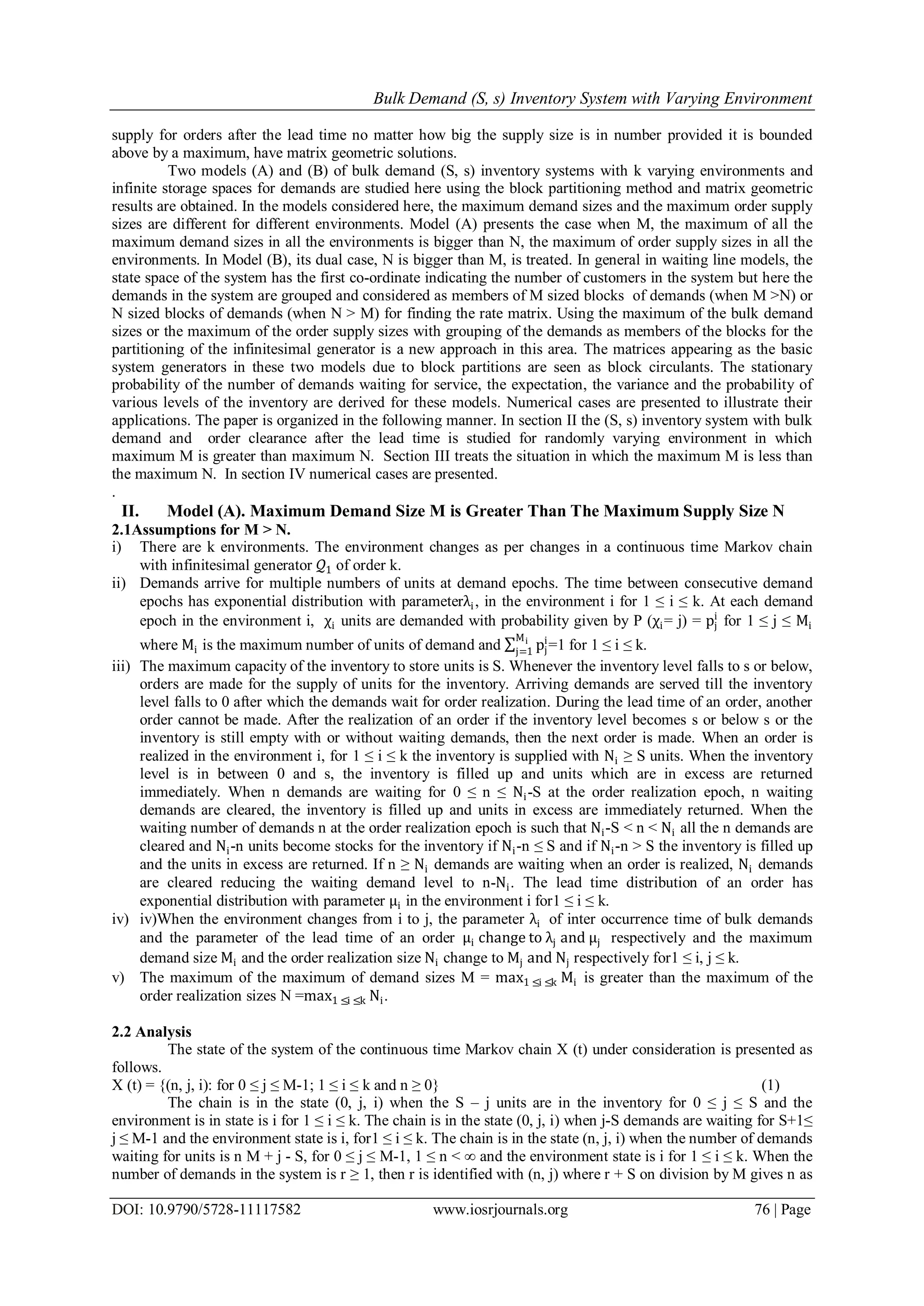
The basic generator 𝒬A
′′
of the system, which is concerned with only the demand and supply, is a matrix
of order Mk given above in (12) where 𝒬A
′′
=A0 + A1 + A2 (13)
Its probability vector w gives, w𝒬A
′′
=0 and w e = 1 (14)
It is well known that a square matrix in which each row (after the first) has the elements of the previous
row shifted cyclically one place right, is called a circulant matrix. It is very interesting to note that the matrix
𝒬A
′′
= A0 + A1 + A2 is a block circulant matrix where each block matrix is rotated one block to the right relative
to the preceding block partition. Let the probability vector of the environment generator 𝒬1 be π. Then π𝒬1 =
0 and π e =1. It can be seen in (13) that the first block-row of type k x Mk is,
W = (𝒬1
′
+ ΛM , Λ1, Λ2 , …ΛM−N−2, ΛM−N−1, ΛM−N + UN, … ΛM−2 + U2, ΛM−1 + U1)
This gives as the sum of the blocks 𝒬1
′
+ ΛM + Λ1+ Λ2 +…. . +ΛM−N−2 + ΛM−N−1 +ΛM−N + UN+…
…+ΛM−2 + U2 + ΛM−1 + U1 =𝒬1. So π 𝒬1 = π 𝒬1
′
+ ΛM + π Λi
M−N−1
i=1 + π (ΛM−i + Ui)N
i=1 = 0 which
implies (π, π… π, π). W = 0 = (π, π… π, π) W’ where W’ is the transpose of vector W. Since all blocks, in any
block-row are seen somewhere in each and every column block due to block circulant structure, the above
equation shows the left eigen vector of the matrix 𝒬A
′′
is (π,π…π). Using (14)
w =
π
M
,
π
M
,
π
M
, … ,
π
M
. (15)
Neuts [8], gives the stability condition as, w A0 e < w A2 e where w is given by (15). Taking the sum
cross diagonally using the structure in (8) and (9) for the A0 and A2 matrices, it can be seen that
w A0 e =
1
M
π nΛn
M
n=1 e =
1
M
π . (λ1E(χ1), λ2E(χ2) , … . , λkE χk ) < w A2 e =
1
M
π( nUn)eN
n=1
=
1
M
π . (μ1M1,μ2M2 , … . , μk MK) .
Taking the probability vector of the environment generator 𝒬1 as π = (π1, π2, … , πk−1, πk) , the
inequality reduces to πi
k
i=1 λiE(χi) < πi μiMi
k
i=1 . (16)
This is the stability condition for (S, s) inventory system under random environment with bulk demand
where maximum of the maximums of demand sizes in all environments is greater than the maximum of order
realization sizes in all environments. When (16) is satisfied, the stationary distribution exists as proved in
Neuts [8].
Let π (n, j, i), for 0 ≤ j ≤ M-1, 1 ≤ i ≤ k and 0 ≤ n < ∞ be the stationary probability of the states in (1)
and πnbe the vector of type 1xMk with, πn= (π(n, 0, 1), π(n, 0, 2) … π(n, 0, k), π(n, 1, 1), π(n, 1, 2),…
π(n, 1, k)... π(n, M-1, 1), π(n, M-1, 2)…π(n, M-1, k) ), for n ≥ 0.
The stationary probability vector 𝜋 = (π0, π1, π3, … … ) satisfies 𝜋QA =0, and 𝜋e=1. (17)
From (17), it can be seen π0B1 + π1A2=0. (18)
πn−1A0+πnA1+πn+1A2 = 0, for n ≥ 1. (19)
Introducing the rate matrix R as the minimal non-negative solution of the non-linear matrix equation
A0+RA1+R2
A2=0, (20)
it can be proved (Neuts [8]) that πn satisfies πn = π0 Rn
for n ≥ 1. (21)
Using (17) and (18), π0 satisfies π0 [B1 + RA2] =0 (22)
Now π0 can be calculated up to multiplicative constant by (22). From (17) and (21) π0 I − R −1
e =1. (23)
Replacing the first column of the matrix multiplier of π0 in equation (22) by the column vector multiplier of π0
in (23), a matrix which is invertible may be obtained. The first row of the inverse of that same matrix is π0 and
this gives along with (21) all the stationary probabilities of the system. The matrix R given in (20) is computed
by substitutions in the recurrence relation
R 0 = 0; R(n + 1) = −A0A1
−1
–R2
(n)A2A1
−1
, n ≥ 0. (24)
The iteration may be terminated to get a solution of R at an approximate level where R n + 1 −
R(n) < ε where ε is very small number.

5. Bulk Demand (S, s) Inventory System with Varying Environment
DOI: 10.9790/5728-11117582 www.iosrjournals.org 79 | Page
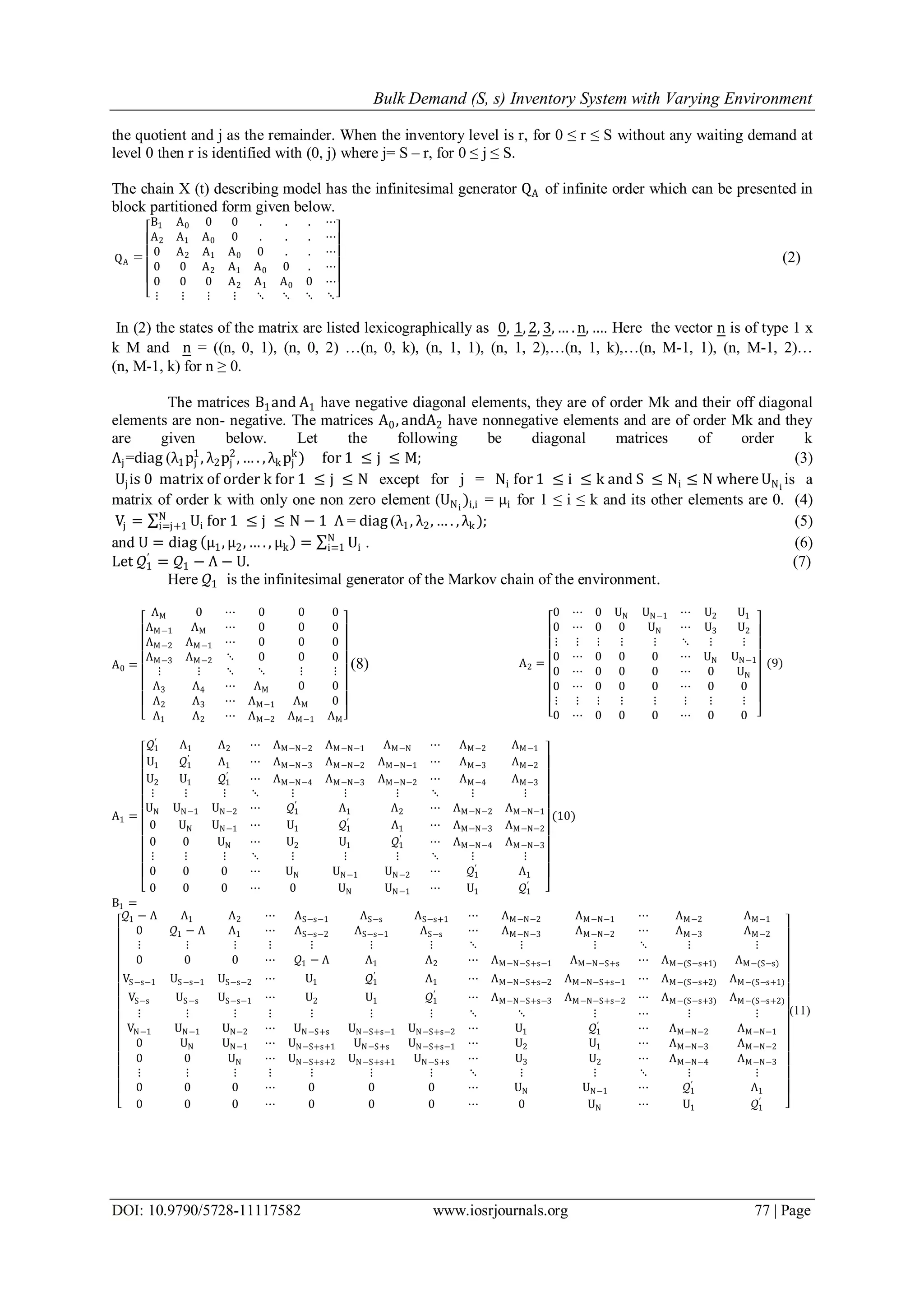
2.3. Performance Measures
(1) The probability of the demand length L = r > 0, P (L = r), can be seen as follows. Let n ≥ 0 and j for 0 ≤ j ≤
M-1 be non-negative integers such that r = n M + j - S. Then using (21) (22) and (23) it is noted that
P (L=r) = 𝜋𝑘
𝑖=1 𝑛, 𝑗, 𝑖 , where r = n M + j - S.
(2) P (waiting demand length = 0) = P (L = 0) = 𝜋𝑘
𝑖=1
𝑆
𝑗=0 (0, j, i) and P (Inventory level is r) = P (INV= r) =
𝜋 0, 𝑆 − 𝑟, 𝑖𝑘
𝑖=1 for 0 ≤ r ≤ S.
(3) The expected demand length E (L), can be calculated as follows. Demand length L = 0 when there is stock in
the inventory or when the inventory becomes empty without a waiting demand. They are described for various
environments in (1) and with probabilities in the elements of 𝜋0 by j for 0 ≤ j ≤ S for n=0. Now for L > 0,
π (n, j, i) = P [L = M n + j - S, and environment state = i], for n ≥ 0, and 0 ≤ j ≤ M-1 and 1 ≤ i ≤ k, which shows
E(L) = 0 P(L=0) + 𝜋𝑘
𝑖=1
𝑀−1
𝑗=𝑆+1 (0,j,i) (j-S) + 𝜋 𝑛, 𝑗, 𝑖𝑘
𝑖=1 𝑀𝑛 + 𝑗 − 𝑆𝑀−1
𝑗=0
∞
𝑛=1
=𝜋0 𝛿1 – S𝜋0 𝛿2+M 𝑛 𝜋 𝑛
∞
𝑛=1 𝑒 + 𝜋 𝑛
∞
𝑛=1 𝛿3- S (1 - 𝜋0 𝑒) where 𝛿1, 𝛿2, 𝑎𝑛𝑑 𝛿3 are type Mk x 1 column
vectors defined as follows. 𝛿1= (0,0,…0,1,1,…1,2,2,…2,…,M-1-S,M-1-S,…,M-1-S)’. Here in the vector, the
number 0 appears (S+1)k times, and the numbers 1,2,3,.., (M-1-S) appear k times one by one in order.
The vector 𝛿2= (0,0,…,0,1,1…1)’ where the number 0 appears (S+1)k times and the number 1 appears (M-1-S)k
times. The vector 𝛿3= (0,0,…0,1,1,…1,2,2,…2,…,M-1, M-1, …, M-1)’ where all the numbers 0 to M-1 appear
k times. On simplification E (L) = 𝜋0 𝛿1 – S𝜋0 𝛿2 +M 𝜋0(I-R)−2
Re + 𝜋0(I-R)−1
R𝛿3- S(1-𝜋0e). (25)
(4) Variance of the demand length can be seen using VAR (L) = E (𝐿2
) – E(L)2
. Let 𝛿4 be column vector
𝛿4 = [0, . .0, 12
, … 12
22
, . . 22
, … 𝑀 − 1−𝑆)2
, … (𝑀 − 1 − 𝑆)2 ′
of type Mkx1 where the number 0 appears
(S+1)k times, and the square of numbers 1,2,3,.., (M-1-S) appear k times one by one in order and let
𝛿5 = [0, . .0, 12
, … 12
22
, . . 22
, … 𝑀 − 1)2
, … (𝑀 − 1)2 ′
of type Mkx1 where the number 0 appears k times,
and the square of numbers 1,2,3,.., (M-1) appear k times one by one in order. It can be seen that the second
moment, E (𝐿2
) = 𝜋𝑘
𝑖=1
𝑀−1
𝑗=𝑆+1 (0, j, i) (j-S)2
+ 𝜋 𝑛, 𝑗, 𝑖𝑘
𝑖=1 [𝑀𝑀−1
𝐽=0 𝑛 + 𝑗∞
𝑛=1 −𝑆]2
. Using Binomial
expansion in the second series it may be noted E (𝐿2
) = 𝜋0 𝛿4 + 𝑀2
𝑛 𝑛 − 1 𝜋 𝑛
∞
𝑛=1 𝑒 + 𝑛𝜋 𝑛
∞
𝑛=1 𝑒 +
𝜋 𝑛
∞
𝑛=1 𝛿5 + 2𝑀 𝑛 𝜋 𝑛 𝛿3
∞
𝑛=1 -2S 𝜋 𝑛, 𝑗, 𝑖𝑘
𝑖=1 𝑀𝑛 + 𝑗𝑀−1
𝑗=0
∞
𝑛=1 + 𝑆2
𝜋 𝑛, 𝑗, 𝑖𝑘
𝑖=1
𝑀−1
𝑗=0
∞
𝑛=1 . After
simplification,
E(𝐿2
)= 𝜋0 𝛿4+𝑀2
[𝜋0(𝐼 − 𝑅)−3
2𝑅2
𝑒 + 𝜋0(𝐼 − 𝑅)−2
𝑅𝑒]+𝜋0(𝐼 − 𝑅)−1
𝑅𝛿5 + 2𝑀 𝜋0(𝐼 − 𝑅)−2
𝑅𝛿3
-2S [M 𝜋0(I-R)−2
Re + 𝜋0(I-R)−1
R𝛿3] +𝑆2
(1-𝜋0 𝑒)
Using (25) and (26) variance of L can be written. (26)
(5) The above partition method may also be used to study the case in which the supply for an order is a finite
valued discrete random variable by suitably redefining the matrices 𝑈𝑗 for 1 ≤ j ≤ N as presented in Rama
Ganesan, Ramshankar and Ramanarayanan for M/M/1 bulk queues. [9].
III. Model.(B). Maximum Demand Size M is Less Than the Maximum Supply Size N
In this Model (B) the dual case of Model (A), namely the case, M < N is treated. (When M =N both
models are applicable and one can use any one of them.) The assumption (v) of Model (A) is modified and all
its other assumptions are unchanged.
3.1Assumption.
v) The maximum of the maximum demands sizes in all the environments M = 𝑚𝑎𝑥1 ≤𝑖 ≤𝑘 𝑀𝑖 is less than the
maximum of the order clearance sizes in all the environments N =𝑚𝑎𝑥1 ≤𝑖 ≤𝑘 𝑁𝑖 where the maximum demands
and order clearance sizes are 𝑀𝑖 and 𝑁𝑖 respectively in the environment i for 1 ≤ i ≤ k.
3.2. Analysis
Since this model is dual, the analysis is similar to that of Model (A). The differences are noted below.
The state space of the chain is defined as follows in a similar way.
X (t) = {(n, j, i): for 0 ≤ j ≤ N-1; 1 ≤ i ≤ k and n ≥ 0} (27)
The chain is in the state (0, j, i) when the S – j units are in the inventory for 0 ≤ j ≤ S and the environment state
is i for 1 ≤ i ≤ k. The chain is in the state (0, j, i) when the inventory is empty and j-S demands are waiting for
order realization where S+1≤ j ≤ N-1 and 1 ≤ i ≤ k. The chain is in the state (n, j, i) when the number of
demands waiting for units is n N + j - S, for 0 ≤ j ≤ N-1, 1 ≤ n < ∞ and the environment state is i for 1 ≤ i ≤ k.
When the number of demands in the system is r ≥ 1, then r is identified with (n, j) where r + S on division by N
gives n as the quotient and j as the remainder. The infinitesimal generator 𝑄 𝐵 of the model has the same block
partitioned structure given in (4) for Model (A) but the inner matrices are of different orders and elements.

6. Bulk Demand (S, s) Inventory System with Varying Environment
DOI: 10.9790/5728-11117582 www.iosrjournals.org 80 | Page
𝑄 𝐵=
𝐵′
1 𝐴′
0 0 0 . . . ⋯
𝐴′
2 𝐴′
1 𝐴′
0 0 . . . ⋯
0 𝐴′
2 𝐴′
1 𝐴′
0 0 . . ⋯
0 0 𝐴′
2 𝐴′
1 𝐴′
0 0 . ⋯
0 0 0 𝐴′
2 𝐴′
1 𝐴′
0 0 ⋯
⋮ ⋮ ⋮ ⋮ ⋱ ⋱ ⋱ ⋱
(28)
In (28) the states of the matrix are listed lexicographically as 0, 1, 2, 3, … . 𝑛, ….Here the state vector is
given as follows. 𝑛 = ((n, 0, 1),…(n, 0, k),(n, 1, 1),…(n, 1, k),(n, 2, 1),…(n, 2, k),…(n, N-1, 1),…(n, N-1, k)),
for 0 ≤ n < ∞. The matrices, 𝐵′1, 𝐴′0 , 𝐴′1 𝑎𝑛𝑑 𝐴′2 are all of order Nk. The matrices 𝐵′1 𝑎𝑛𝑑 𝐴′1 have negative
diagonal elements and their off diagonal elements are non- negative. The matrices 𝐴′0 𝑎𝑛𝑑 𝐴′2 have nonnegative
elements. They are all given below. As in model (A), letting 𝛬𝑗 , 𝑓𝑜𝑟 1 ≤ 𝑗 ≤ 𝑀 , 𝑎𝑛𝑑 𝑈𝑗 , 𝑉𝑗 𝑓𝑜𝑟 1 ≤ 𝑗 ≤ 𝑁,
Λ and U as matrices of order k given by (3), (4), (5) and (6) and letting 𝒬1
′
= 𝒬1 − 𝛬 − 𝑈, the partitioning
matrices are defined as follows
𝐴′
0 =
0 0 ⋯ 0 0 0 ⋯ 0
⋮ ⋮ ⋯ ⋮ ⋮ ⋮ ⋮ ⋮
0 0 ⋯ 0 0 0 ⋯ 0
𝛬 𝑀 0 ⋯ 0 0 0 ⋯ 0
𝛬 𝑀−1 𝛬 𝑀 ⋯ 0 0 0 ⋯ 0
⋮ ⋮ ⋱ ⋮ ⋮ ⋮ ⋮ ⋮
𝛬2 𝛬3 ⋯ 𝛬 𝑀 0 0 ⋯ 0
𝛬1 𝛬2 ⋯ 𝛬 𝑀−1 𝛬 𝑀 0 ⋯ 0
29 𝐴′2 =
𝑈 𝑁 𝑈 𝑁−1 𝑈 𝑁−2 ⋯ 𝑈3 𝑈2 𝑈1
0 𝑈 𝑁 𝑈 𝑁−1 ⋯ 𝑈4 𝑈3 𝑈2
0 0 𝑈 𝑁 ⋯ 𝑈5 𝑈4 𝑈3
0 0 0 ⋱ 𝑈6 𝑈5 𝑈4
⋮ ⋮ ⋮ ⋱ ⋮ ⋮ ⋮
0 0 0 ⋯ 𝑈 𝑁 𝑈 𝑁−1 𝑈 𝑁−2
0 0 0 ⋯ 0 𝑈 𝑁 𝑈 𝑁−1
0 0 0 ⋯ 0 0 𝑈 𝑁
(30)
𝐴′1 =
𝒬1
′
𝛬1 𝛬2 ⋯ 𝛬 𝑀 0 0 ⋯ 0 0
𝑈1 𝒬1
′
𝛬1 ⋯ 𝛬 𝑀−1 𝛬 𝑀 0 ⋯ 0 0
𝑈2 𝑈1 𝒬1
′
⋯ 𝛬 𝑀−2 𝛬 𝑀−1 𝛬 𝑀 ⋯ 0 0
⋮ ⋮ ⋮ ⋱ ⋮ ⋮ ⋮ ⋱ ⋮ ⋮
𝑈 𝑁−𝑀−1 𝑈 𝑁−𝑀−2 𝑈 𝑁−𝑀−3 ⋯ 𝒬1
′
𝛬1 𝛬2 ⋯ 𝛬 𝑀−1 𝛬 𝑀
𝑈 𝑁−𝑀 𝑈 𝑁−𝑀−1 𝑈 𝑁−𝑀−2 ⋯ 𝑈1 𝒬1
′
𝛬1 ⋯ 𝛬 𝑀−2 𝛬 𝑀−1
𝑈 𝑁−𝑀+1 𝑈 𝑁−𝑀 𝑈 𝑁−𝑀−1 ⋯ 𝑈2 𝑈1 𝒬1
′
⋯ 𝛬 𝑀−3 𝛬 𝑀−2
⋮ ⋮ ⋮ ⋱ ⋮ ⋮ ⋮ ⋱ ⋮ ⋮
𝑈 𝑁−2 𝑈 𝑁−3 𝑈 𝑁−4 ⋯ 𝑈 𝑁−𝑀−2 𝑈 𝑁−𝑀−3 𝑈 𝑁−𝑀−2 ⋯ 𝒬1
′
𝛬1
𝑈 𝑁−1 𝑈 𝑁−2 𝑈 𝑁−3 ⋯ 𝑈 𝑁−𝑀−1 𝑈 𝑁−𝑀−2 𝑈 𝑁−𝑀−1 ⋯ 𝑈1 𝒬1
′
(31)
𝒬 𝐵
′′
=
𝒬1
′
+ 𝑈 𝑁 𝛬1 + 𝑈 𝑁−1 ⋯ 𝛬 𝑀−1 + 𝑈 𝑁−𝑀+1 𝛬 𝑀 + 𝑈 𝑁−𝑀 𝑈 𝑁−𝑀−1 ⋯ 𝑈2 𝑈1
𝑈1 𝒬1
′
+ 𝑈 𝑁 ⋯ 𝛬 𝑀−2 + 𝑈 𝑁−𝑀+2` 𝛬 𝑀−1 + 𝑈 𝑁−𝑀+1 𝛬 𝑀 + 𝑈 𝑁−𝑀 ⋯ 𝑈3 𝑈2
⋮ ⋮ ⋮⋮⋮ ⋮ ⋮ ⋮ ⋮⋮⋮ ⋮ ⋮
𝑈 𝑁−𝑀−2 𝑈 𝑁−𝑀−3 ⋯ 𝒬1
′
+ 𝑈 𝑁 𝛬1 + 𝑈 𝑁−1 𝛬2 + 𝑈 𝑁−2 ⋯ 𝛬 𝑀 + 𝑈 𝑁−𝑀 𝑈 𝑁−𝑀−1
𝑈 𝑁−𝑀−1 𝑈 𝑁−𝑀−2 ⋯ 𝑈1 𝒬1
′
+ 𝑈 𝑁 𝛬1 + 𝑈 𝑁−1 ⋯ 𝛬 𝑀−1 + 𝑈 𝑁−𝑀+1 𝛬 𝑀 + 𝑈 𝑁−𝑀
𝛬 𝑀 + 𝑈 𝑁−𝑀 𝑈 𝑁−𝑀−1 ⋯ 𝑈2 𝑈1 𝒬1
′
+ 𝑈 𝑁 ⋯ 𝛬 𝑀−2 + 𝑈 𝑁−𝑀+2 𝛬 𝑀−1 + 𝑈 𝑁−𝑀+1
⋮ ⋮ ⋮⋮⋮ ⋮ ⋮ ⋮ ⋮⋮⋮ ⋮ ⋮
𝛬2 + 𝑈 𝑁−2 𝛬3 + 𝑈 𝑁−3 ⋯ 𝑈 𝑁−𝑀−1 𝑈 𝑁−𝑀−2 𝑈 𝑁−𝑀−3 ⋯ 𝒬1
′
+ 𝑈 𝑁 𝛬1 + 𝑈 𝑁−1
𝛬1 + 𝑈 𝑁−1 𝛬2 + 𝑈 𝑁−2 ⋯ 𝛬 𝑀 + 𝑈 𝑁−𝑀 𝑈 𝑁−𝑀−1 𝑈 𝑁−𝑀−2 ⋯ 𝑈1 𝒬1
′
+ 𝑈 𝑁
(33)
The basic generator (33) which is concerned with only the demands and supply is 𝒬 𝐵
′′
= 𝐴′0 + 𝐴′1 +
𝐴′2. This is also block circulant. Using similar arguments given for Model (A) it can be seen that its probability
vector is
𝜋
𝑁
,
𝜋
𝑁
,
𝜋
𝑁
, … ,
𝜋
𝑁
and the stability condition remains the same. Following the arguments given for Model
(A), one can find the stationary probability vector for Model (B) also in matrix geometric form. All performance
measures given in section 2.3 including the expectation of waiting demands for supply and its variance for
Model (B) have the same form as given in Model (A) except M is replaced by N.

7. Bulk Demand (S, s) Inventory System with Varying Environment
DOI: 10.9790/5728-11117582 www.iosrjournals.org 81 | Page
IV. Numerical Illustration
Six numerical examples are studied to exhibit the usefulness of this above study since so far bulk
demand inventory models have not been treated at any depth. The results obtained in the examples are presented
in table 1. The varying environment considered here has three states whose infinitesimal generator is
𝒬1 =
−3 1 2
2 −3 1
1 2 −3
. In the six cases the maximum capacity of the inventory and the ordering level are S=5
and s=2. The lead time parameter 𝜇 = (3, 4, 5) for the three environments. The maximum demand size is 8 in the
first four examples and the demand size probabilities in the three environments (i=1, 2, 3), P (𝜒𝑖= j) = 𝑝𝑗
𝑖
for 1≤ j
≤ 8 are given by 𝑝1
1
= .5, 𝑝5
1
= .4 and 𝑝8
1
= .1; 𝑝1
2
= .6, 𝑝5
2
= .3, 𝑝8
2
= .1; 𝑝1
3
=.7, 𝑝5
3
= .2, 𝑝8
3
= .1 and 𝑝𝑗
𝑖
= 0 for i = 1,2,3
and j ≠ 1,5,8. In the last two examples the maximum demand size is 5 and the demand size probabilities in the
three environments (i=1,2,3), P(𝜒𝑖=j)=pj
i
for 1≤ j ≤ 5 are given by p1
1
= .5, p5
1
= .5 ; p1
2
= .6, p5
2
= .4 ; p1
3
=.7, p5
3
= .3
and pj
i
= 0 for i = 1,2,3 and j ≠ 1,5. The maximum supply for an order after the lead time is N= 8 in examples
1,2,5,6 and N=7 in examples 3 and 4. For three cases (M=8, N=8), (M=8, N=7) and (M=5, N=8) two sets arrival
rates for bulk demands are considered as follows λ= (2, 3, 4) and λ = (3, 4, 5) respectively.
Using the theory mentioned, fifteen iterations are performed to find the rate matrix R to present the probabilities
and various performance measures. The various inventory level probabilities P(S=i) for 1 ≤ i ≤ 5, probability of
empty stock and empty queue P(S=0,L=0), queue length probabilities for L=1, L=2 and for various ranges, the
expected queue length of demands, the variances and standard deviations obtained are listed. Figure 1 compares
the results obtained for the six examples.
Table1. Performance Measures
λ=(2,3,4),
M=8,N=8
λ=(3,4,5),
M=8,N=8
λ=(2,3,4),
M=8,N=7
λ =(3,4,5),
M=8,N=7
λ=(2,3,4),
M=5,N=8
λ=(3,4,5),
M=5,N=8
Norm 0 0.000001 0 0.000001 0 0
P(S=5) 0.269622 0.219981 0.26065 0.210089 0.359018 0.318294
P(S=4) 0.207264 0.17197 0.205028 0.168154 0.233524 0.209436
P(S=3) 0.161299 0.136563 0.162088 0.13585 0.156201 0.142097
P(S=2) 0.05346 0.054522 0.0553 0.055719 0.04548 0.049533
P(S=1) 0.023172 0.027688 0.024909 0.029284 0.017267 0.022354
P(S=0, L=0) 0.046097 0.049506 0.046132 0.0494 0.053424 0.061912
P(L=1) 0.042828 0.047583 0.043132 0.047672 0.04312 0.051824
P(L=2) 0.035658 0.041055 0.036269 0.041553 0.030437 0.037623
π 1e = P(3≤ L ≤ 10) 0.128616 0.175832 0.132342 0.180817 0.054615 0.088512
π2e= P(11≤ L ≤ 18) 0.025489 0.052471 0.027033 0.055906 0.0063 0.01569
π3e=P(19≤ L ≤ 26) 0.005175 0.015903 0.005649 0.017533 0.000554 0.00229
π 4e =P(27≤ L ≤ 33) 0.001052 0.004824 0.001182 0.005503 0.000056 0.000368
π (n>3)=P( L ≥ 27 ) 0.00132 0.006926 0.001495 0.008022 0.000062 0.000435
P(L ≥ 0) 0.285183 0.389276 0.292025 0.400903 0.18851 0.258285
P(1≤ S ≤5) 0.714817 0.610724 0.707975 0.599097 0.81149 0.741715
E(L) 0.914466 1.980259 0.971758 2.13345 0.122178 0.439724
VAR(L) 52.143939 99.496507 54.70922 106.202096 17.177379 33.288072
Std(L) 7.221076028 9.974793582 7.396568 10.30544 4.14456 5.769582
Figure1. Probabilities of Waiting Length of Demands.
V. Conclusion
The (S, s) inventory system with bulk demand under varying environment has been studied. The
difficulties involved in finding the stationary demand length probabilities are resolved by considering the
maximum of the demands and the supply sizes for partitions of the infinitesimal generator. Using the Matrix

8. Bulk Demand (S, s) Inventory System with Varying Environment
DOI: 10.9790/5728-11117582 www.iosrjournals.org 82 | Page
partition method of Neuts, the demand length probabilities have been presented for bulk demand (S, s) inventory
system with randomly varying environment explicitly using the rate matrix. Various performance measures are
derived. Two general models are presented considering the demand size is bigger than the supply size and the
supply size is bigger than the demand size. Numerical examples are treated to illustrate the usefulness of the
method. For future studies, models with catastrophic demands and supplies may present further useful results.
Acknowledgement
The first author thanks ANSYS Inc., USA, for providing facilities. The contents of the article published are the
responsibilities of the authors.
References
[1]. Thangaraj.V and Ramanarayanan.R, (1983), An operating policy in inventory system with random lead times and unit demands,
Math.Oper and Stat.Series Optimization, Vol1 p111-124.
[2]. Daniel,J.K and Ramanarayanan.R, (1988) An S-s Inventory system with rest periods to the server, Naval Research Logistics
Quarterly,Vol.35,pp119-123.
[3]. Ayyappan.G, Muthu Ganapathy Subramanian. A and Gopal Sekar. (2010). M/M/1 retrial queueing system with loss and feedback
under pre- emptive priority service, IJCA, 2, N0.6,-27-34.
[4]. D. Bini, G. Latouche, and B. Meini. (2005). Numerical methods for structured Markov chains, Oxford Univ. Press, Oxford.
[5]. Chakravarthy.S.R and Neuts. M.F.(2014). Analysis of a multi-server queueing model with MAP arrivals of customers, SMPT, Vol
43, 79-95,
[6]. Gaver, D., Jacobs, P and Latouche, G, (1984). Finite birth-and-death models in randomly changing environments. AAP.16, 715–731
[7]. Latouche.G, and Ramaswami.V, (1998). Introduction to Matrix Analytic Methods in Stochastic Modeling, SIAM. Philadelphia.
[8]. Neuts.M.F.(1981).Matrix-Geometric Solutions in Stochastic Models: An algorithmic Approach, The Johns Hopkins Press,
Baltimore
[9]. Rama Ganesan, Ramshankar and Ramanarayanan,(2014) M/M/1 Bulk Arrival and Bulk Service Queue with Randomly Varying
Environment, IOSR-JM, Vol. 10, Issue 6,Ver.III, pp. 58-66.
[10]. Sundar Viswanathan, (2014) Stochastic Analysis of Static and Fatigue Failures with Fluctuating Manpower and Business, IJCA,
Vol. 106, No.4, Nov. pp.19-23.
[11]. William J. Stewart, The matrix geometric / analytic methods for structured Markov Chains, N.C State University
www.sti.uniurb/events/sfmo7pe/slides/Stewart-2 pdf.
[12]. Rama Ganesan and Ramanarayanan (2014), Stochastic Analysis of Project Issues and Fixing its Cause by Project Team and
Funding System Using Matrix Analytic Method, IJCA, Vol.107, No.7, pp.22-28.