Briaud2001

114 / JOURNAL OF GEOTECHNICAL AND GEOENVIRONMENTAL ENGINEERING / FEBRUARY 2001
MULTIFLOOD AND MULTILAYER METHOD FOR SCOUR RATE
PREDICTION AT BRIDGE PIERS
By J. L. Briaud,1
Fellow, ASCE, H. C. Chen,2
Member, ASCE,
K. W. Kwak,3
Student Member, ASCE, S. W. Han,4
and F. C. K. Ting,5
Member, ASCE
ABSTRACT: The SRICOS method was proposed in 1999 to predict the scour depth versus time curve at a
cylindrical bridge pier for a constant velocity flow, a uniform soil, and a deep-water condition. In this article,
the method is extended to include a random velocity-time history and a multilayer soil stratigraphy; it is called
the Extended-SRICOS or E-SRICOS. The algorithms to accumulate the effects of different velocities and to
sequence through a series of soil layers are described. The procedure followed by the computer program to step
into time is outlined. A simplified version of E-SRICOS called S-SRICOS is also presented; calculations for the
S-SRICOS method can easily be done by hand. Eight bridges in Texas are used as case histories to compare
predictions by the two new methods (E-SRICOS and S-SRICOS) with measurements at the bridge sites.
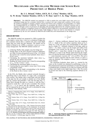
FIG. 1. Schematic Diagram and Result of EFA (Erosion Func-
tion Apparatus) (Briaud et al. 1999)
SRICOS METHOD
The SRICOS method was proposed in 1999 to predict the
scour depth z– versus time t curve at a cylindrical bridge pier
for a constant velocity flow, a uniform soil, and a water depth
larger than two times the pier diameter. The details can be
found in Briaud et al. (1999); a summary is given as a nec-
essary background. The SRICOS method consists of:
1. Collecting Shelby tube samples near the bridge pier
2. Testing them in the EFA (Erosion Function Apparatus;
see ͗http://tti.tamu.edu/geotech/scour͘) (Fig. 1) to obtain
the erosion rate z˙– (mm/h) versus hydraulic shear stress ␶
(N/m2
) curve
3. Calculating the maximum hydraulic shear stress ␶max
around the pier before scour starts
4. Reading the initial erosion rate z˙–i (mm/h) corresponding
to ␶max on the z˙– versus ␶ curve
5. Calculating the maximum depth of scour z˙–max
6. Constructing the scour depth z– versus time t curve using
a hyperbolic model
7. Reading the scour depth corresponding to the duration
of the flood on the z– versus t curve
In the EFA, the Shelby tube is placed vertically through a
tight-fitting hole in the bottom of a pipe with a rectangular
cross section. The Shelby tube is kept flush with the bottom
of the pipe but the soil sample is pushed out of the Shelby
tube by a piston and protrudes 1 mm into the pipe (Fig. 1).
Water flows through the pipe at a velocity v, and the time t
required to erode the 1 mm of soil is recorded. The erosion
rate is z˙– = 1/t in mm/h and the hydraulic shear stress ␶
(N/m2
) imposed by the water on the soil is calculated by using
the Moody Chart (Moody 1944):
1
Spencer J. Buchanan Prof., Dept. of Civ. Engrg., Texas A&M Univ.,
College Station, TX 77843-3136.
2
Assoc. Prof., Dept. of Civ. Engrg., Texas A&M Univ., College Sta-
tion, TX.
3
Grad. Student, Dept. of Civ. Engrg., Texas A&M Univ., College Sta-
tion, TX.
4
Grad. Student, Dept. of Civ. Engrg., Texas A&M Univ., College Sta-
tion, TX.
5
Assoc. Prof., Dept. of Civ. Engrg., South Dakota State Univ., Brook-
ings, SD 57006.
Note. Discussion open until July 1, 2001. Separate discussions should
be submitted for the individual papers in this symposium. To extend the
closing date one month, a written request must be filed with the ASCE
Manager of Journals. The manuscript for this paper was submitted for
review and possible publication on November 16, 1999. This paper is
part of the Journal of Geotechnical and Geoenvironmental Engineer-
ing, Vol. 127, No. 2, February, 2001. ᭧ASCE, ISSN 1090-0241/01/0002-
0114–0125/$8.00 ϩ $.50 per page. Paper No. 22144.
1 2
␶ = f ␳v (1)
8
where f = friction coefficient obtained from the roughness
ε/D; ε = depth of the soil surface asperities taken as D50/2,
where D50 is the soil grain size corresponding to 50% pass-
ing by weight; D = hydraulic diameter of the pipe, taken as
(2ab/a ϩ b), where a and b are the height and width of the
rectangular cross section for the pipe; ␳ = density of water
(kg/m3
); and v = mean flow velocity in the pipe (m/s). The
coefficient f is read on the Moody Chart knowing the rough-
ness ε/D and the Reynold’s number R, which is (vD/␯) where
␯ = water kinematic viscosity (10Ϫ6
m2
/s at 20ЊC). The soil is
tested at various velocities and for each velocity a z˙– and a ␶
value are obtained. The complete z˙– versus ␶ curve is obtained
in this fashion.
The maximum hydraulic shear stress ␶max exerted by the
water on the riverbed was obtained by performing a series of
three-dimensional numerical simulations of water flowing past
a cylindrical pier of diameter B on a flat river bottom and with
a large water depth (water depth larger than 1.5B). The results
of several runs lead to the following equation (Briaud et al.
1999):
J. Geotech. Geoenviron. Eng. 2001.127:114-125.
Downloadedfromascelibrary.orgbyNewYorkUniversityon02/19/15.CopyrightASCE.Forpersonaluseonly;allrightsreserved.

JOURNAL OF GEOTECHNICAL AND GEOENVIRONMENTAL ENGINEERING / FEBRUARY 2001 / 115
FIG. 2. Example of SRICOS Method
1 12
␶ = 0.094␳v Ϫ (2)max ͩ ͪlog R 10
where ␳ = density of water (kg/m3
); v = the depth average
velocity in the river at the location of the pier if the bridge
was not there [obtained by performing a hydrologic analysis
with a computer program such as HEC-RAS (1997)]; and R
is (vB/␯), where B = pier diameter and ␯ = kinematic viscosity
of water (10Ϫ6
m2
/s at 20ЊC). There is no scatter associated
with (2), because it is based on a theoretical simulation. The
initial rate of scour z˙–i is read on the z˙– versus ␶ curve from the
EFA test at the value of ␶max.
The maximum depth of scour z–max was obtained by perform-
ing a series of 43 model scale flume tests (36 tests on three
different clays and 7 tests in sand) (Briaud et al. 1999). The
results of these experiments and a review of other work lead
to the following equation, which appears to be equally valid
for clays and sands:
0.635
z– (mm) = 0.18R (3)max
R has the same definition in (3), as in (2). The regression
coefficient for (3) was 0.74. The equation that describes the
shape of the scour depth z– versus time t curve is
t
z– = (4)
1 t
ϩ
˙z– z–maxi
where z˙–i and z–max have been previously defined. This hyper-
bolic equation was chosen because it fits well the curves ob-
tained in the flume tests. Once the duration t of the flood to
be simulated is known, the corresponding z– value is calculated
using (4). If z˙–i is large as it is in clean fine sands, then z– is
close to z–max even for small t values. But if z˙–i is small as it
can be in clays, then z– may only be a small fraction of z–max.
An example of the SRICOS method is shown in Fig. 2.
In the design of the foundation, the predicted scour depth z–
is added to the pile length required to safely carry the foun-
dation load. Assuming that the scour depth will always reach
z–max during the life of the bridge is uneconomical when the
soil scours very slowly. This was the incentive for the devel-
opment of SRICOS. The method, as described in the previous
paragraphs, is limited to a constant velocity hydrograph (v =
constant), a uniform soil (one z˙– versus ␶ curve), and a rela-
tively deep water depth. In reality, rivers create varying ve-
locity hydrographs and soils are layered. The following de-
scribes how SRICOS was extended to include these two
features. The case of shallow water flow (water depth over
pier diameter <2), noncircular piers, and flow directions dif-
ferent from the pier main axis are not addressed in this article.
SMALL FLOOD FOLLOWED BY BIG FLOOD
The velocity versus time history for a river over many years
is very different from a constant velocity history. In order to
investigate the influence of the difference between the two
velocity histories or hydrographs on the depth of scour at a
bridge pier, the case of a sequence of two different yet constant
velocity floods scouring a uniform soil was first considered
(Fig. 3). Flood 1 has a velocity v1 and lasts a time t1, while
the subsequent flood 2 has a larger velocity v2 and lasts a time
t2. The scour depth z– versus time t curve for flood 1 is de-
scribed by
t
z– = (5)
1 t
ϩ
˙z– z–max1i1
For flood 2, the z– versus t curve is
t
z– = (6)
1 t
ϩ
˙z– z–i 2 max 2

FIG. 4. Multiflood Flume Experiment Results: (a) Floods and
Flood Sequence in Experiments; (b) Experiment Result for
Flood 1 Alone; (c) Experiment Result for Flood 2 Alone; (d) Ex-
periment Result for Flood 1 and 2 Sequence Shown in (a) and
Prediction for Flood 2
TABLE 1. Properties of Porcelain Clay for Flume Experiment
Property
number
(1)
Property
(2)
Value
(3)
1 Liquid limit, % 34.4
2 Plastic limit, % 20.2
3 Plasticity index, % 14.1
4 Specific gravity 2.61
5 Water content, % 28.5
6 Mean diameter D50, mm 0.0062
7 Sand content, % 0.0
8 Silt content, % 75.0
9 Clay content, % 25.0
10 Shear strength, kPa (lab. vane) 12.5
11 CEC, meq/100 g 8.30
12 SAR 5.00
13 pH 6.00
14 Electrical conductivity, mmhos/cm 1.20
15 Unit weight, kN/m3
18.0
FIG. 3. Scour due to Sequence of Two Flood Events (Small
Flood Followed by Big Flood)
After a time t1, flood 1 creates a scour depth z–1, given by (5)
[Point A on Fig. 3(b)]. This depth z–1 would have been created
in a shorter time t* by flood 2, because v2 is larger than v1
[point B on Fig. 3(c)]. This time t* can be found by setting
(5) with z– = z–1 and t = t1 equal to (6) with z– = z–1 and t = t*:
t1
t* = (7)
˙z– 1 1i 2
˙ϩ t z– Ϫ1 ͩ ͪi 2
˙z– z– z–max1 max2i1
When flood 2 starts, event though the scour depth z–1 was due
to flood 1 over a time t1, the situation is identical to having
had flood 2 for a time t*. Therefore when flood 2 starts, the
scour depth versus time curve proceeds from point B on Fig.
3(c) until point C after a time t2. The z– versus t curve for the
sequence of flood 1 and 2 follows the path OA on the curve
for flood 1, then switches to BC on the curve for flood 2. This
is shown as the curve OAC on Fig. 3(d).
A set of two experiments was conducted to investigate this
reasoning. For these experiments, a 25 mm diameter pipe was
placed in the middle of a flume. The pipe was pushed through
150 mm thick deposit of clay made by placing prepared blocks
of clay side by side in a tight arrangement. The properties of
the clay are listed in Table 1. The water depth was 400 mm
and the mean flow velocity was v1 = 0.3 m/s in flood 1 and
v2 = 0.4 m/s for flood 2 [Fig. 4(a)]. The first of the two ex-
periments consisted of setting the velocity equal to v2 for 100
h and recording the z– versus t curve [Fig. 4(c)]. The second
of the two experiments consisted of setting the velocity equal
to v1 for 115 h [Fg. 4(b)] and then switching to v2 for 100 h
[Fig. 4(d)]. Also shown in Fig. 4(d) is the prediction of the
portion of the z– versus t curve under the velocity v2 according
to the procedure described in Fig. 4. As can be seen, the pre-
diction is very reasonable.
BIG FLOOD FOLLOWED BY SMALL FLOOD AND
GENERAL CASE
Flood 1 has a velocity v1 and lasts t1 [Fig. 5(a)]. It is fol-
lowed by flood 2, which has a velocity v2 smaller than v1 and
lasts t2. The scour depth z– versus time t curve is given by
(5) for flood 1 and by (6) for flood 2. After a time t1, flood
1 creates a scour depth z–1. This depth z–1 is compared with
z–max 2; if z–1 is larger than z–max 2, then, when flood 2 starts, the
scour hole is already larger than it can be with flood 2, there-
fore, flood 2 cannot create additional scour and the scour depth
versus time curve remains flat during flood 2. If z–1 is smaller
than z–max 2, then the procedure followed for the case of a small
flood followed by a big flood applies and the combined curve
is as shown in Fig. 5.
In the general case, the velocity versus time history exhibits
many sequences of small floods and big floods. The calcula-
tions for scour depth are performed by choosing an increment
of time ⌬t and breaking the complete velocity versus time
history into a series of partial flood events each lasting ⌬t. The
first two floods in the hydrograph are handled by using the
procedure of Fig. 3 or Fig. 5, depending on the case. Then the
process advances by stepping into time and considering a new
flood 2 and a new t* at each step. The time ⌬t is typically
one day and a velocity versus time history can be 50 years

FIG. 5. Scour due to Sequence of Two Flood Events (Big
Flood Followed by Small Flood)
FIG. 7. Scour of Two-Layer Soil (Soft Layer over Hard Layer)
FIG. 6. Scour of Two-Layer Soil (Hard Layer over Soft Layer)
long. The many steps of calculations are handled with a com-
puter program called SRICOS. The output of the program is
the depth of scour versus time curve over the duration of the
velocity versus time history.
HARD SOIL LAYER OVER SOFT SOIL LAYER
The original SRICOS method (Briaud et al. 1999) was de-
veloped for a uniform soil. In order to investigate the influence
of the difference between a uniform soil and a more realistic
layered soil on the depth of scour at a bridge pier, the case of
a two layer soil profile scoured by a constant velocity flood
was considered (Fig. 6). Layer 1 is hard and ⌬z–1 thick, layer
2 underlays layer 1 and is softer than layer 1. The scour depth
z– versus time t curve for layer 1 is given by (5) [Fig. 6(a)],
and the z– versus t curve for layer 2 is given by (6) [Fig. 6(b)].
If ⌬z–1 is larger than the maximum depth of scour in layer 1,
z–max1, then the scour process is contained in layer 1 and does
not reach layer 2. If, however, the scour depth reaches ⌬z–1
[point A in Fig. 6(a)], layer 2 starts to be eroded. In this case,
even though the scour depth ⌬z–1 was due to the scour of layer
1 over a time t1, at that time the situation is identical to having
had layer 2 scoured over a time t* [point B in Fig. 6(b)].
Therefore, when layer 2 starts being eroded, the scour versus
depth curve proceeds from point B to point C in Fig. 6(b).
The combined curve for the two-layer system is OAC, as given
in Fig. 6(c).
SOFT SOIL LAYER OVER HARD SOIL LAYER AND
GENERAL CASE
Layer 1 is soft and ⌬z–1 thick; layer 2 underlays layer 1 and
is harder than layer 1. The scour depth z– versus time t curve
for layer 1 is given by (5) [Fig. 7(a)], and the z– versus t curve
for layer 2 is given by (6) [Fig. 7(b)]. If ⌬z–1 is larger than the
maximum depth of scour in layer 1, z–max1, then the scour pro-
cess is contained in layer 1 and does not reach layer 2. If,
however, the scour depth reaches ⌬z–1 [point A in Fig. 7(a)],
layer 2 starts to erode. In this case, even though the scour
depth ⌬z–1 was due to the scour of layer 1 over a time t1, at
that time the situation is identical to having had layer 2 soured
over an equivalent time t* [point B in Fig. 7(b)]. Therefore,
when layer 2 starts being eroded, the scour versus depth curve
proceeds from point B to point C in Fig. 7(b). The combined
curve for the two layer system is OAC, as given in Fig. 7(c).
In the general case, there may be a series of soil layers with
different erosion functions. The computations proceed by step-
ping forward in time. The time steps are ⌬t long, the velocity
is the one for the corresponding flood event, and the erosion
function (z˙– versus t) is the one for the soil layer corresponding
to the current scour depth (bottom of the scour hole). When
⌬t is such that the scour depth proceeds to a new soil layer,
the computations follow the process described in Figs. 6 or 7,
depending on the case. The calculations are handled by the

TABLE 2. Equivalent Time te and Selected Parameters
Bridge
(1)
thydro
(years)
(2)
vmax
(m/s)
(3)
z˙i,mean
(mm/h)
(4)
te
(h)
(5)
Navasota, bent 3 5 1.90 8.91 165.40
10 1.98 8.91 214.08
15 2.06 8.91 243.60
20 2.06 8.91 251.02
25 2.06 8.91 267.66
30 2.06 8.91 267.93
35 2.06 8.91 322.35
41 2.54 8.91 274.05
Navasota, bent 5 5 3.16 22.39 125.99
10 3.24 22.39 333.94
15 3.31 22.39 442.69
20 3.31 22.39 448.07
25 3.31 22.39 468.58
30 3.31 22.39 468.58
35 3.31 22.39 596.67
41 3.82 22.39 427.89
Brazos, bent 3 5 4.20 65.26 540.97
10 4.20 65.26 543.37
15 4.20 65.26 595.91
20 4.20 65.26 595.91
25 4.20 65.26 595.91
33 4.20 65.26 812.01
San Jacinto, bent 43 5 1.73 17.44 271.86
10 3.07 17.44 196.25
Trinity, bent 3 5 1.40 50.60 137.74
10 1.40 50.60 146.29
15 2.00 50.60 280.21
17 2.00 50.60 292.96
Trinity, bent 4 5 3.22 39.82 257.28
10 3.22 39.82 309.94
15 4.06 39.82 311.93
17 4.06 39.82 368.93
San Marcos, bent 9 5 1.12 61.75 25.42
10 1.12 61.75 25.78
15 1.50 61.75 39.97
20 1.50 61.75 43.47
25 1.50 61.75 44.84
30 1.50 61.75 46.55
35 1.50 61.75 49.85
40 1.50 61.75 51.66
Sims, bent 3 3 0.95 2.69 152.84
Bedias 75, bent 26 5 2.15 127.44 103.53
10 2.17 127.44 143.49
15 2.17 127.44 161.32
20 2.17 127.44 188.14
25 2.17 127.44 224.44
30 2.17 127.44 263.28
35 2.17 127.44 263.28
40 2.17 127.44 281.80
45 2.19 127.44 289.03
50 2.19 127.44 289.03
Bedias 90, bent 6 5 1.36 44.25 65.36
10 1.37 44.25 109.04
15 1.54 44.25 103.68
18 1.54 44.25 104.26FIG. 8. Velocity Hydrographs: (a) Constant; (b) True Hydro-
graph (Both Hydrographs Would Lead to Same Scour Depth)
same SRICOS program as the one mentioned for the velocity
hydrograph. The output of the program is the scour depth ver-
sus time for the multilayered soil system and for the complete
velocity hydrograph.
EQUIVALENT TIME
The computer program SRICOS is required to predict the
scour depth versus time curve as explained in the preceding
section. An attempt was made to simplify the method to the
point where only hand calculations would be needed. This re-
quires the consideration of an equivalent uniform soil and an
equivalent time for a constant velocity history. The equivalent
uniform soil is characterized by an average z˙– versus ␶ curve
over the anticipated scour depth. The equivalent time te is the
time required for the maximum velocity in the hydrograph to
create the same scour depth as the one created by the complete
hydrograph (Fig. 8). The equivalent time te was obtained for
55 cases generated from eight bridge sites. For each bridge
site, soil samples were collected in Shelby tubes and tested in
the EFA to obtain the erosion function z˙– versus ␶, then the
hydrograph was collected from the nearest gauge station and
the SRICOS program was used to calculate the scour depth.
That scour depth was entered in (4) along with the correspond-
ing z˙–i and z–max to get te. The z˙–i value was obtained from an
average z˙– versus ␶ curve within the ﬁnal scour depth by read-
ing the z˙– value which corresponded to ␶max obtained from (2).
In (2), the pier diameter B and the maximum velocity vmax
found to exist in the hydrograph over the period considered
were used. The z–max value was obtained from (3) while using
B and vmax for the pier Reynolds number. The hydrograph at
each bridge was also divided in shorter period hydrographs,
and for each period an equivalent time te was calculated. This
generated the 55 cases listed in Table 2.
The equivalent time was then correlated to the duration of
the hydrograph thydro, the maximum velocity in the hydrograph
vmax, and the initial erosion rate z˙–i. These quantities are listed
in Table 2. A multiple regression on that data gave the follow-
ing relationship:
0.126 1.706 Ϫ0.20
˙t (h) = 73(t (years)) (v (m/s)) (z– (mm/h)) (8)e hydro max i
The regression coefﬁcient for (8) was 0.77. This time te can
then be used in (4) to calculate the scour at the end of the
hydrograph. A comparison between the scour depth predicted
by the Extended-SRICOS method using the complete hydro-
graph and the Simple-SRICOS method using the equivalent
time is shown in Fig. 9.

FIG. 9. Comparison of Scour Depth Using Extended-SRICOS
and Simple-SRICOS Methods
FIG. 10. Examples of Discharge Hydrographs: (a) Brazos
River at US90A; (b) San Marcos River at SH80; (c) Sims Bayou at
SH35
EXTENDED-SRICOS METHOD AND SIMPLE-SRICOS
METHOD
For final design purposes the Extended-SRICOS method
(E-SRICOS) is used to predict the scour depth z– versus time
t over the duration of the design hydrograph. The method pro-
ceeds as follows:
1. Calculate the maximum depth of scour z–max for the design
velocity using (3).
2. Collect samples at the site within the depth z–max.
3. Test the samples in the EFA to obtain the erosion func-
tions (z˙– versus ␶) for the layers involved.
4. Prepare the flow hydrograph for the bridge. This step
may consist in downloading the discharge hydrograph
from a USGS (United States Geological Survey) gauge
station near the bridge (Fig. 10). These discharge hydro-
graphs can be found on the Internet at the USGS web
site, ͗www.usgs.gov͘. The discharge hydrograph then
needs to be transformed into a velocity hydrograph (Figs.
11–13). This transformation is performed using a pro-
gram such as HEC-RAS (1997), which makes use of the
transversed river bottom profile at the bridge site to link
the discharge Q (m3
/s) to the velocity v (m/s) at the an-
ticipated location of the bridge pier.
5. Use the SRICOS program (Kwak et al. 1999) with the
following input: the z˙– versus ␶ curves for the various
layers involved; the velocity hydrograph v versus t, the
pier diameter B, the viscosity of the water ␯, and the
density of the water ␳w. Note that the water depth y is
not an input, because at this time the solution is limited
to a ‘‘deep water’’ condition. This condition is realized
when y Ն 1.5B; indeed beyond this water depth, the
scour depth becomes independent of the water depth
(Melville and Coleman 1999; p. 197).
6. The SRICOS program steps into time by making use of
the original SRICOS method and the accumulation al-
gorithms described in Figs. 3, 5, 6, and 7. The usual time
step ⌬t is one day, because that is the usual reading fre-
quency of the USGS gauges. The duration of the hydro-
graph can vary from a few days to over 100 years.
7. The output of the program is the depth of scour versus
time over the period covered by the hydrograph (Figs.
11–13).
For predicting the future development of a scour hole at a
bridge pier over a design life tlife, one can either develop a
synthetic hydrograph much like is done in the case of earth-
quakes or assume that the hydrograph recorded over the last
period equal to tlife will repeat itself. The time required to per-
form step 3 is about eight hours per Shelby tube sample, be-
cause it takes about eight points to properly describe the ero-
sion function (z˙– versus ␶ curve) and for each point the water
is kept flowing for one hour to get a good average z˙– value.
The time required to perform all other steps, except for step
2, is about four hours for someone who has done it before. In
order to reduce these four hours to a few minutes, a simplified
version of SRICOS called S-SRICOS was developed. One
must understand that this simplified version is only recom-
mended for preliminary design purposes. If S-SRICOS shows
clearly that there is no need for refinement, then there is no
need for E-SRICOS; if not, one must perform an E-SRICOS
analysis.
For preliminary design purposes, the simple SRICOS
method (S-SRICOS) can be used. The method proceeds as
follows:
1. Calculate the maximum depth of scour z–max for the design
velocity vmax using (3). The design velocity is usually the
one corresponding to the 100 year flood or the 500 year
flood.
2. Collect samples at the site within the depth z–max.
3. Test the samples in the EFA to obtain the erosion func-
tion (z˙– versus ␶) for the layers involved.
4. Create a single equivalent erosion function by averaging
the erosion functions within the anticipated depth of
scour.
5. Calculate the maximum shear stress ␶max around the pier
before scour starts using (2). In (2), use the pier diameter
B and the design velocity vmax.

FIG. 11. Velocity Hydrograph and Scour Depth versus Time
Curve for Bent 3 of Brazos River Bridge at US90A
Curve for Bent 3 of San Marcos River Bridge at SH80
Curve for Bent 3 of Sims Bayou River Bridge at SH35
6. Read the erosion rate z˙–i corresponding to ␶max on the
equivalent function.
7. Calculate the equivalent time te for a given design life
of the bridge thydro for the design velocity ␯max and for the
z˙–i value of step 6 using (8).
8. Knowing te, z˙–i, and z–max, calculate the scour depth z– at
the end of the design life using (4).
An example of such calculations is shown in Fig. 14.
CASE HISTORIES
In order to evaluate the E-SRICOS and S-SRICOS methods,
eight bridges were selected (Table 3). These bridges all satis-
fied the following requirements: (1) the predominant soil type
was fine grained soils according to existing borings; (2) the
river bottom profiles were measured at two dates separated by
at least several years; (3) these river bottom profiles indicated
anywhere from 0.05 to 4.57 m of scour; (4) a USGS gauging
station existed near the bridge; and (5) drilling access was
relatively easy. Fig. 15 shows where the bridges are located.
The Navasota River bridge at SH7 was built in 1956. The
main channel bridge has an overall length of 82.8 m and con-
sists of three continuous steel girder main spans with four
concrete pan girder approach spans. The foundation type is
steel piling down to 5.5 m below the channel bed, which con-
sists of silty and sandy clay down to the bottom of the piling
according to existing borings. Between 1956 and 1996 the
peak flood took place in 1992 and generated a measured flow
of 1,600 m3
/s, which corresponds to a HEC-RAS calculated
mean approach flow velocity of 3.9 m/s at bent 5 and 2.6
m/s at bent 3. The pier at bent 3 was square with a side equal
to 0.36 m, while the pier at bent 5 was 0.36 m wide, 8.53 m
long, and had a square nose. The angle between the flow di-
rection and the pier main axis was 5Њ for bent 5. River bottom
profiles exist for 1956 and 1996 and show 0.76 m of local
scour at bent 3 and 1.8 m of total scour at bent 5. At bent 5
the total scour was made up of 1.41 m of local scour and 0.39
m of contraction scour, as explained later.
The Brazos River bridge at US90A was built in 1965. The
bridge has an overall length of 287 m and consists of three

FIG. 14. Example of Scour Calculations by S-SRICOS Method
TABLE 3. Full-Scale Bridges as Case Histories
continuous steel girder main spans with eight prestressed con-
crete approach spans. The foundation type is concrete piling
penetrating 9.1 m below the channel bed, which consists of
sandy clay, clayey sand, and sand down to the bottom of the
piling, according to existing borings. Between 1965 and 1998
the peak flood occurred in 1966 and generated a measured
flow of 2,600 m3
/s, which corresponded to a HEC-RAS cal-
culated mean approach velocity of 4.2 m/s at bent 3. The pier
at bent 3 was 0.91 m wide, 8.53 m long, and had a round
nose. The pier was in line with the flow. River bottom profiles

FIG. 15. Location of Case History Bridges
FIG. 16. Erosion Function for San Jacinto River Sample (7.6–
8.4 m depth)
exist for 1965 and 1997 and show 4.43 m of total scour at
bent 3 made up of 2.87 m of local scour and 1.56 m of com-
bined contraction and general scour, as explained later.
The San Jacinto River bridge at US90 was built in 1988.
The bridge is 1,472.2 m long and has 48 simple prestressed
concrete beam spans and three continuous steel plate girder
spans. The foundation type is concrete piling penetrating 24.4
m below the channel bed at bent 43, where the soil consists
of clay, silty clay, and sand down to the bottom of the piles
according to existing borings. Between 1988 and 1997, the
peak flood took place in 1994 and generated a measured flow
of 10,000 m3
/s, which corresponded to a HEC-RAS calculated
mean approach velocity of 3.1 m/s at bent 43. The pier at bent
43 was square with a side equal to 0.85 m. The angle between
the flow direction and the pier main axis was 15Њ. River bot-
tom profiles exist for 1988 and 1997 and show 3.17 m of total
scour at bent 43 made up of 1.47 m of local scour and 1.70
m of combined contraction and general scour, as explained
later.
The Trinity River bridge at FM787 was built in 1976. The
bridge has three main spans and three approach spans, with
an overall length of 165.2 m. The foundation type is timber
piling and the soil is sandy clay to clayey sand. Between 1976
and 1993, the peak flood took place in 1990 and generated a
measured flow of 2,950 m3
/s, which corresponded to a HEC-
RAS calculated mean approach flow velocity of 2.0 m/s at
bent 3 and 4.05 m/s at bent 4. The piers at bent 3 and 4 were
0.91 m wide, 7.3 m long, and had a round nose. The angle
between the flow direction and the pier main axis was 25Њ.
River bottom profiles exist for 1976 and for 1992 and show
4.57 m of total scour at both bent 3 and bent 4 made up of
2.17 m of local scour and 2.40 m of contraction and general
scour, as explained later.
The San Marcos River bridge at SH80 was built in 1939.
This 176.2 m long bridge has 11 prestressed concrete spans.
The soil tested from the site is a low plasticity clay. Between
1939 and 1998, the peak flood occurred in 1992 and generated
a measured flow of 1,0009 m3
/s, which corresponds to a HEC-
bent 9. The pier at bent 9 is 0.91 m wide, 14.2 m long, and
has a round nose. The pier is in line with the flow. River
bottom profiles exist for 1939 and 1998 and show 2.66 m of
total scour at bent 9, made up of 1.27 m of local scour and
1.39 m of contraction and general scour, as explained later.
The Sims Bayou bridge at SH35 was built in 1993. This
85.3 m long bridge has five spans. Each bent rests on four
drilled concrete shafts. Soil borings indicate mostly clay layers
with a significant sand layer about 10 m thick starting at a
depth of approximately 4 m. Between 1993 and 1996, the peak
flood occurred in 1994 and generated a measure flow of 200
m3
/s, which corresponds to a HEC-RAS calculated mean ap-
proach flow velocity of 0.93 m/s at bent 3. The pier at bent 3
is circular with a 0.76 m diameter. The angle between the flow
direction and the pier main axis was 5Њ. River bottom profiles
exist for 1993 and 1995 and indicate 0.05 m of local scour at
bent 3.
The Bedias Creek bridge at US75 was built in 1947. This
271.9 m long bridge has 29 spans, and bent 26 is founded on
a spread footing. The soil tested from the site varied from low
plasticity clay to fine silty sand. Between 1947 and 1996, the
peak flood occurred in 1991 and generated a measured flow
of 650 m3
/s, which corresponds to a HEC-RAS calculated
mean approach flow velocity of 2.15 m/s at bent 26. The pier
at bent 26 is square with a side of 0.86 m. The pier is in line
with the flow. River bottom profiles exist for 1947 and 1996
and show 2.13 m of total scour at bent 26 made up of 1.35 m
of local scour and 0.78 m of contraction and general scour, as
explained later.
The Bedias Creek bridge at SH90 was built in 1979. This
73.2 m long bridge is founded on 8 m long concrete piles
embedded in layers of sandy clay and firm gray clay. Between
1979 and 1996, the peak flood occurred in 1991 and generated
a measured flow of 650 m3
/s, which corresponds to a HEC-
bent 6. The pier at bent 6 was square with a side of 0.38 m.
The angle between the flow direction and the pier main axis
was 5Њ. River bottom profiles exist for 1979 and 1996 and
show 0.61 m of local scour at bent 6.
PREDICTED AND MEASURED LOCAL SCOUR FOR
EIGHT BRIDGES
For each bridge, the E-SRICOS and the S-SRICOS methods
were used to predict the local scour at the chosen bridge pier
location. One pier was selected for each bridge except for the
Navasota River bridge at SH7 and the Trinity River bridge at
FM787, for which two piers were selected. Therefore, a total
of 10 predictions were made for these eight bridges. These
predictions are not Class A predictions, since the measured
values were known before the prediction process started. How-
ever, the predictions were not modified once they were ob-
tained.
For each bridge, Shelby tube samples, were taken near the
bridge pier within a depth at least equal to two pier widths
below the pier base. The boring location was chosen to be as
close as practically possible to the bridge pier considered. The

TABLE 4. Soil Properties at Bridge Sites
FIG. 17. Erosion Function for Bedias Creek River Sample
(6.1–6.9 m Depth)
distance between the pier and the boring varied from 2.9 to
146.3 m (Table 3). In all instances the boring data available
was studied in order to infer the relationship between the soil
layers at the pier and at the sampling locations. Shelby tube
samples to be tested were selected as the most probable rep-
resentative samples at the bridge pier. These samples were
tested in the EFA and yielded erosion functions z˙– versus ␶.
Figs. 16 and 17 are examples of the erosion functions ob-
tained. The samples were also analyzed for common soil prop-
erties (Table 4).
For each bridge, the USGS gauge data was obtained from
the USGS Internet site. This data consisted of a record of
discharge Q versus time t over the period of time separating
the two river bottom profile observations (Fig. 10). This dis-
charge hydrograph was transformed into a velocity hydrograph
using the program HEC-RAS (HEC-RAS 1997) and proceed-
ing as follows. The input to HEC-RAS is the bottom profile
of the river cross section (obtained from the Texas DOT rec-
ords), the mean longitudinal slope of the river at the bridge
site (obtained from topographic maps; Table 3), and Manning’s
roughness coefficient [estimated at 0.035 for all cases, after
Young et al. (1997)]. For a given discharge Q, HEC-RAS
gives the velocity distribution in the river cross section, in-
cluding the mean approach velocity v at the selected pier lo-
cation. Many runs of HEC-RAS for different values of Q are
used to develop a relationship between Q and v. The relation-
ship (regression equation) is then used to transform the Q-t
hydrograph into the v-t hydrograph at the selected pier (Figs.
11–13).
Next, the program SRICOS (Kwak et al. 1999) was used to
predict the scour depth z– versus time t curve. For each bridge,
the input consisted of the z˙– versus ␶ curves (erosion functions)
for each layer at the bridge pier (e.g., Figs. 16 and 17), the v
versus t record (velocity hydrograph) (e.g., Figs. 11–13), the
pier diameter B, the viscosity of the water ␯, and the density
of the water ␳w. The output of the program was the scour depth
z– versus time t curve for the selected bridge pier (e.g., Figs.
11–13), with the predicted local scour depth corresponding to
the last value on the curve.
The measured local scour depth was obtained for each case
history by analyzing the two bottom profiles of the river cross
section (e.g., Figs. 18 and 19). This analysis was necessary to
separate the scour components which added to the total scour
at the selected pier. The two components were local scour and
contraction/general scour. This separation was required be-
cause, at this time, SRICOS only predicts the local scour. The
contraction/general scour over the period of time separating
the two river bottom profiles was calculated as the average
scour over the width of the channel. This width was taken as
the width corresponding to the mean flow level (width AB on
Figs. 18 and 19). Within this width, the net area between the
two profiles was calculated with scour being positive and ag-
gradation being negative. The net area was then divided by
the width AB to obtain an estimate of the mean contraction/
general scour. Once this contraction/general scour was ob-
tained, it was subtracted from the total scour at the bridge pier
to obtain the local scour at the bridge pier. Note that in some
instances there was no need to evaluate the contraction/general
scour. This is the case of bent 3 for the Navasota Bridge (Fig.
18). Indeed, in this case the bent was in the dry at the time of
the field visit (flood plain) and the local scour could be mea-
sured directly. Fig. 20 shows the comparison between E-
SRICOS predicted and measured values of local scour at the
bridge piers. The precision and accuracy of the method appear
reasonably good. On one hand, one would wish to have more

FIG. 18. Profiles of Navasota River Bridge at SH7
FIG. 19. Profiles of Brazos River Bridge at US90A
than 10 data points; on the other hand, these 10 data points
are 10 full scale real situations.
The S-SRICOS method was performed next. For each
bridge pier the maximum depth of scour z–max was calculated
using (3). The velocity used for (3) was the maximum velocity
that occurred during the period of time separating the two river
bottom profile observations. Then, at each pier an average ero-
sion function (z˙– versus ␶ curve) within the maximum scour
depth was generated. Then, the maximum shear stress ␶max
around the pier before scour starts was calculated using (2)
and assuming that the pier was circular (Table 3). The initial
scour rate z˙–i was read on the average erosion function for that
pier (Table 3). The equivalent time te was calculated by (8),
using thydro equal to the time separating the two river bottom
profile observations and vmax equal to the maximum velocity
that occurred during thydro (Table 3). Knowing te, z˙–i, and z–max,
the scour depth accumulated during the period of thydro was
calculated using (4). Fig. 21 is a comparison between the mea-
sured values of local scour and the predicted values using the
S-SRICOS method. The precision and accuracy of the method
appear reasonably good. One must keep in mind that the 10
case histories used to evaluate the S-SRICOS method are the
same cases that were used to develop that method. Therefore,
this does not represent an independent evaluation. All the de-
tails of the prediction process can be found in Kwak et al.
(1999).
Note that at this time E-SRICOS and S-SRICOS do not in-
clude correction factors for pier shape, skew angle between the

FIG. 20. Predicted versus Measured Local Scour for E-
SRICOS Method
FIG. 21. Predicted versus Measured Local Scour for S-
SRICOS Method
flow direction and the pier main axis, and shallow water depth
effects. Such factors exist (Richardson and Davis 1995; Melville
and Coleman 1999) but were derived for sands and not for
clays. Research continues to develop such factors for clays.
CONCLUSIONS
A method is proposed to predict the depth of the local scour
hole versus time curve around a bridge pier in a river for a
given velocity hydrograph and for a layered soil system. The
method is limited at this time to cylindrical piers and water
depths larger than two times the pier width. The prediction
process makes use of a new flood accumulation principle and
a new layer equivalency principle. These are incorporated in
a computer program called SRICOS, used to generate the
scour versus time curve. A simplified version of this method
is also proposed and only requires hand calculations. The sim-
plified method can be used for preliminary design purposes.
Both methods are evaluated by comparing predicted scour
depths and measured scour depths for 10 piers at eight full-
scale bridges. The precision and accuracy of both methods
appear good. Research is continuing to extend this method to
other scour problems.
ACKNOWLEDGMENTS
This project was sponsored by the Texas Department of Transportation,
where David Stolpa, Tony Schneider, Mark McClelland, Melinda
Luna, Kim Culp, Peter Smith, and Jay Vose were very helpful and sup-
portive. This research effort is continuing under the sponsorship of
the National Cooperative Highway Research Program, where Tim Hess is
the contact person. At the Federal Highway Administration, Sterling
Jones provided valuable background information. The writers also
wish to thank Rao Gudavalli, Gengsheng Wei, and Bertrans Philogene for
their contribution to the study as graduate students at Texas A&M Uni-
versity.
APPENDIX. REFERENCES
Briaud, J.-L., Ting, F. C. K., Chen, H. C., Gudavalli, R., Perugu, S., and
Wei, G. (1999). ‘‘SRICOS: prediction of scour rate in cohesive soils
at bridge piers.’’ J. Geotech. and Geoenvir. Engrg., ASCE, 125(4),
237–246.
HEC-RAS: Hydrologic Engineering Center–River Analysis System user’s
manual, version 2.0. (1997). U.S. Army Corps of Engineers, Davis,
Calif.
Kwak, K., Briaud, J.-L., Chen, C. H., Han, S. W., and Ting, F. C. K.
(1999). ‘‘The SRICOS method for predicting local scour at bridge
piers.’’ Res. Rep. Prepared for the Texas Dept. of Transp. on Project
2937, Texas A&M University, College Station, Tex.
Melville, B. W., and Coleman, S. E. (1999). Bridge scour, Water Resource
Publications, Highlands Ranch, Colo.
Moody, L. F. (1944). ‘‘Friction factors for pipe flow.’’ Trans. Am. Soc. of
Mech. Engrs., 66.
Richardson, E. V., and Davis, S. R. (1995). ‘‘Hydraulic Engineering Cir-
cular No. 18.’’ Rep. No. FHWA-IP-90-017, Federal Highway Admin-
istration, Washington, D.C.
Young, D. F., Munson, B. R., and Okisshi, T. H. (1997). A brief intro-
duction to fluid mechanics, Wiley, New York.

Briaud2001

Recommended

Recommended

More Related Content

What's hot

What's hot (20)

Similar to Briaud2001

Similar to Briaud2001 (20)

Recently uploaded

Recently uploaded (20)

Briaud2001