Downloaded 28 times


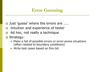
![Error Guessing
Defects’ histories are useful
Some items to try are:
Empty or null lists/strings
Zero instances/occurrences
Blanks or null characters in strings
Negative numbers
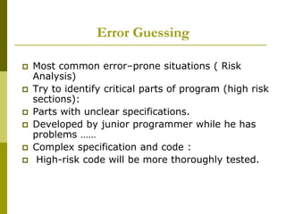
“Probability of errors remaining in the program is
proportional to the number of errors that have
been found so far” [Myers 79]](https://image.slidesharecdn.com/blackbox-191116054136/85/Black-Box-Testing-27-320.jpg)

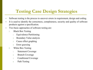
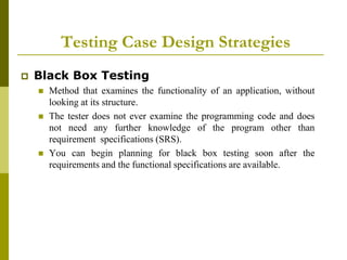
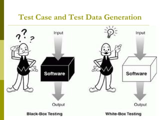
The document outlines software testing strategies, focusing on black box and white box testing approaches, including their advantages and disadvantages. It discusses test case generation techniques such as equivalence class partitioning and boundary value analysis, which help identify potential errors through systematic input categorization. Additionally, it presents practical examples and guidelines for designing test cases to ensure effective testing of software functionalities.