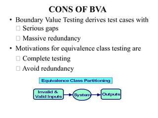
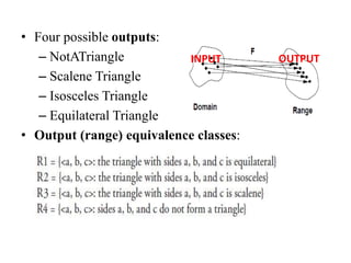
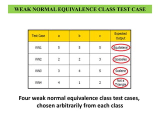
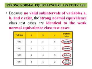
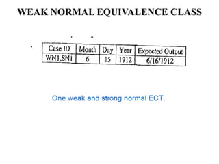
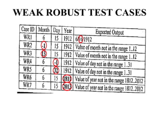
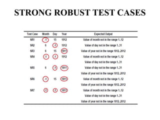
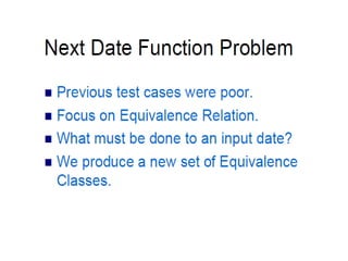
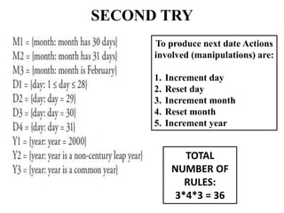
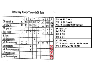
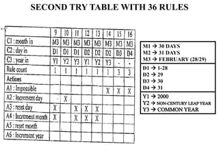
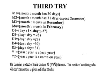
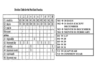
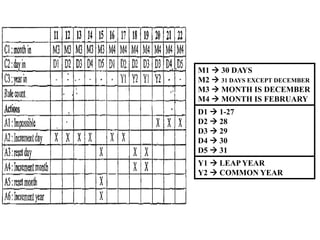
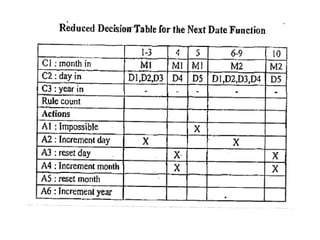
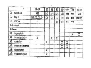
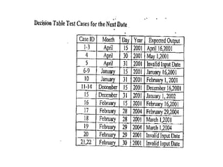
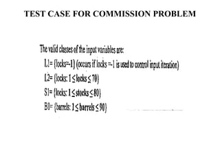
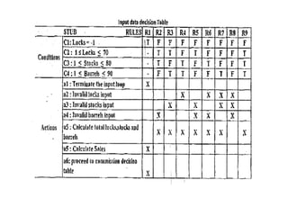
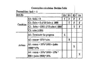
This document provides an overview of black box testing techniques, specifically boundary value analysis, equivalence class testing, and decision table testing. It discusses unit testing in procedural and object-oriented programming. For boundary value analysis, it defines the technique and provides examples testing valid and invalid input boundaries. Equivalence class testing partitions the input domain into classes where members of a class are considered equivalent. Decision table testing systematically tests all combinations of input conditions and expected outputs.

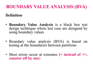
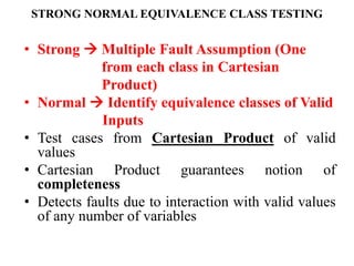
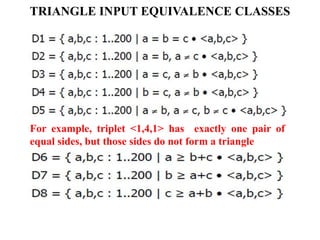
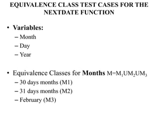
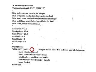
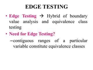
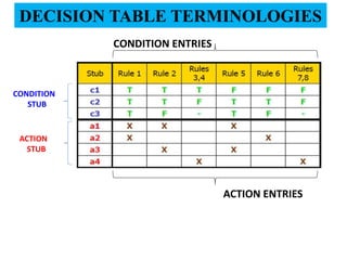
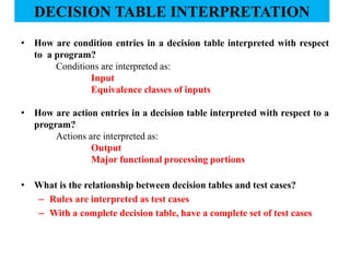
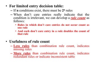
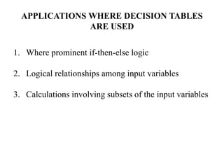
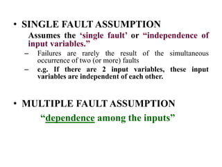
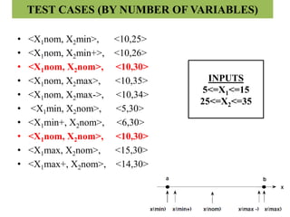
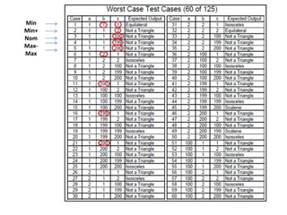
![• When a function F is implemented as a
program, the input variables x1 and x2 will
have some boundaries:
a <= x1 <=b
c <= x2 <=d
where
- [a,b] and [c,d] are the intervals
BVA focuses on the boundary of the input
space to identify test cases](https://image.slidesharecdn.com/boundaryvalueanalysisequivalentclasspartitiondecisiontable-200927060915/85/Software-Testing-Boundary-Value-Analysis-Equivalent-Class-Partition-Decision-Table-9-320.jpg)

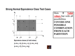
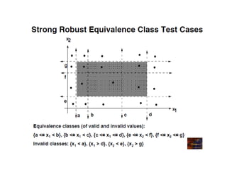
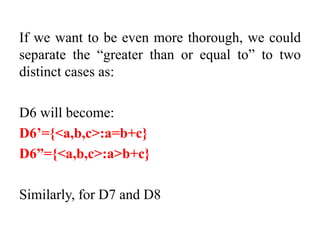
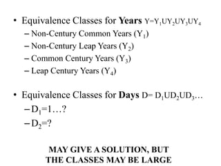
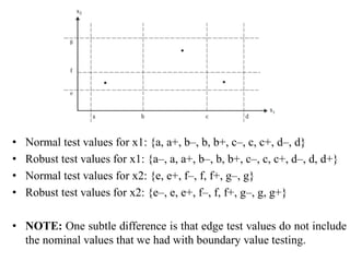
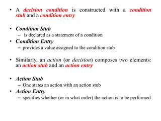
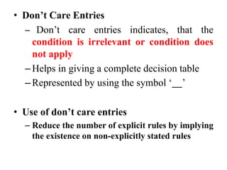
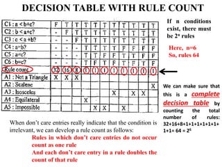
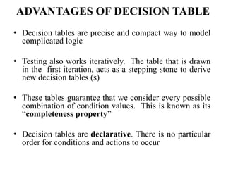
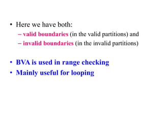
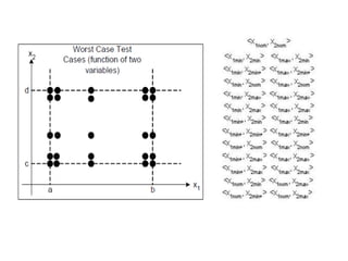
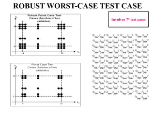
![ROBUSTNESS TEST CASES FOR A FUNCTION
OF TWO VARIABLES
Dots that are outside the range
[a, b] of variable x1.
Similarly, for variable x2, we have
crossed its legitimate boundary of
[c, d] of variable x2.](https://image.slidesharecdn.com/boundaryvalueanalysisequivalentclasspartitiondecisiontable-200927060915/85/Software-Testing-Boundary-Value-Analysis-Equivalent-Class-Partition-Decision-Table-23-320.jpg)
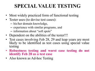
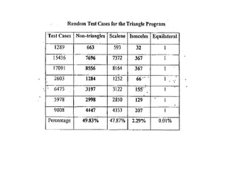
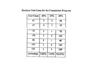
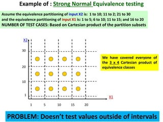
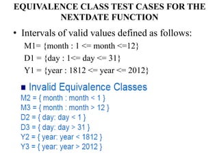
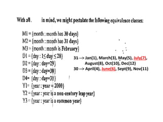
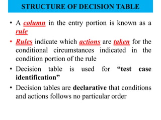
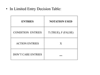
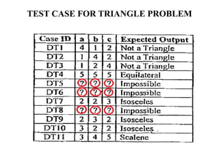
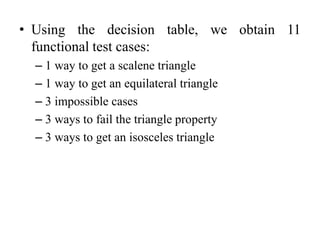
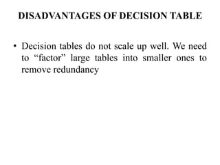
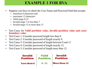
![RANDOM TESTING
• Basic idea is that, rather than always choose the
min, min+, nom, max-, and max values of a
bounded variable, use a random number
generator to pick test case values
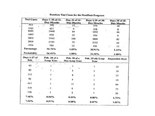
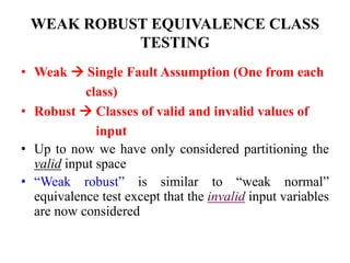
• In Visual Basic application, to pick values for a
bounded variable a<=x<=b, uses
x=Int((b-a+1)*Rnd+a)
where,
Int Returns the integer part of floating
point number
Rnd Function generates random numbers
in the interval [0,1]](https://image.slidesharecdn.com/boundaryvalueanalysisequivalentclasspartitiondecisiontable-200927060915/85/Software-Testing-Boundary-Value-Analysis-Equivalent-Class-Partition-Decision-Table-36-320.jpg)