The document discusses classification techniques, focusing on the naïve bayes classifier, its principles, and applications in various fields such as life sciences and security. It explains the difference between supervised and unsupervised classification, the formal definition of classification problems, and the use of Bayes' theorem for probabilistic classification. Additionally, it highlights various classification techniques, including statistical-based methods, distance-based classification, decision trees, and machine learning approaches.

1. Classification: Naïve Bayes’ Classifier

2. Today’s discussion…
 Introduction to Classification
 Classification Techniques
 Supervised and unsupervised classification
 Formal statement of supervised classification technique
 Bayesian Classifier
 Principle of Bayesian classifier
 Bayes’ theorem of probability
 Naïve Bayesian Classifier
2

3. 3
A Simple Quiz: Identify the objects

4. Introduction to Classification
4
Example8.1
 Teacher classify students as A, B, C, D and F based on their marks. The
following is one simple classification rule:
Mark ≥ 𝟗𝟎 : A
𝟗𝟎 > Mark ≥ 𝟖𝟎 : B
8𝟎 >Mark ≥ 𝟕𝟎 :C
𝟕𝟎 >Mark ≥ 𝟔𝟎 :D
6𝟎 >Mark : F
Note:
Here, we apply the above rule to a specific data
(in this case a table of marks).

5. Examples of Classification in Data Analytics
5
 Life Science: Predicting tumor cells as benign or malignant
 Security: Classifying credit card transactions as legitimate or
fraudulent
 Prediction: Weather, voting, political dynamics, etc.
 Entertainment: Categorizing news stories as finance, weather,
entertainment, sports, etc.
 Social media: Identifying the current trend and future growth

6. Classification : Definition
6
 Classification is a form of data analysis to extract models describing
important data classes.
 Essentially, it involves dividing up objects so that each is assigned to one of
a number of mutually exhaustive and exclusive categories known as
classes.
 The term “mutually exhaustive and exclusive” simply means that each object
must be assigned to precisely one class
 That is, never to more than one and never to no class at all.

7. Classification Techniques
7
 Classification consists of assigning a class label to a set of unclassified
cases.
 Supervised Classification
 The set of possible classes is known in advance.
 Unsupervised Classification
 Set of possible classes is not known. After classification we can try to assign a
name to that class.
 Unsupervised classification is called clustering.

8. Supervised Classification
CS 40003: Data Analytics 8

9. Unsupervised Classification
9

10. Supervised Classification Technique
10
 Given a collection of records (training set )
 Each record contains a set of attributes, one of the attributes is the
class.
 Find a model for class attribute as a function of the values of
other attributes.
 Goal: Previously unseen records should be assigned a class as
accurately as possible.
 Satisfy the property of “mutually exclusive and exhaustive”

11. Illustrating Classification Tasks
11
Apply
Model
Induction
Deduction
Learn
Model
Model
Tid Attrib1 Attrib2 Attrib3 Class
1 Yes Large 125K No
2 No Medium 100K No
3 No Small 70K No
4 Yes Medium 120K No
5 No Large 95K Yes
6 No Medium 60K No
7 Yes Large 220K No
8 No Small 85K Yes
9 No Medium 75K No
10 No Small 90K Yes
10
Tid Attrib1 Attrib2 Attrib3 Class
11 No Small 55K ?
12 Yes Medium 80K ?
13 Yes Large 110K ?
14 No Small 95K ?
15 No Large 67K ?
10
Test Set
Learning
algorithm
Training Set

12. Classification Problem
12
 More precisely, a classification problem can be stated as below:
Given a database D = 𝑡1, 𝑡2, … . . , 𝑡𝑚 of tuples and a set of classes C =
𝑐1, 𝑐2, … . . , 𝑐𝑘 , the classification problem is to define a mapping f ∶ D → 𝐶,
Where each 𝑡𝑖 is assigned to one class.
Note that tuple 𝑡𝑖 ∈ 𝐷 is defined by a set of attributes 𝐴 = 𝐴1, 𝐴2, … . . , 𝐴𝑛 .
Definition 8.1: Classification Problem

13. Classification Techniques
13
 A number of classification techniques are known, which can be broadly
classified into the following categories:
1. Statistical-Based Methods
• Regression
• Bayesian Classifier
2. Distance-Based Classification
• K-Nearest Neighbours
3. Decision Tree-Based Classification
• ID3, C4.5, CART
5. Classification using Machine Learning (SVM)
6. Classification using Neural Network (ANN)

14. Classification Techniques
14
 A number of classification techniques are known, which can be broadly
classified into the following categories:
1. Statistical-Based Methods
• Regression
• Bayesian Classifier
2. Distance-Based Classification
• K-Nearest Neighbours
3. Decision Tree-Based Classification
• ID3, C4.5, CART
5. Classification using Machine Learning (SVM)
6. Classification using Neural Network (ANN)

15. Bayesian Classifier
15

16. Bayesian Classifier
16
 Principle
 If it walks like a duck, quacks like a duck, then it is probably a duck

17.  A statistical classifier
 Performs probabilistic prediction, i.e., predicts class membership probabilities
 Foundation
 Based on Bayes’ Theorem.
 Assumptions
1. The classes are mutually exclusive and exhaustive.
2. The attributes are independent given the class.
 Called “Naïve” classifier because of these assumptions.
 Empirically proven to be useful.
 Scales very well.
17
Bayesian Classifier

18. Example: Bayesian Classification
18
 Example 8.2: Air Traffic Data
 Let us consider a set
observation recorded in a
database
 Regarding the arrival of airplanes
in the routes from any airport to
New Delhi under certain
conditions.

19. Air-Traffic Data
19
Days Season Fog Rain Class
Weekday Spring None None On Time
Weekday Winter None Slight On Time
Weekday Winter None None On Time
Holiday Winter High Slight Late
Saturday Summer Normal None On Time
Weekday Autumn Normal None Very Late
Holiday Summer High Slight On Time
Sunday Summer Normal None On Time
Weekday Winter High Heavy Very Late
Weekday Summer None Slight On Time
Cond. to next slide…

20. Air-Traffic Data
20
Days Season Fog Rain Class
Saturday Spring High Heavy Cancelled
Weekday Summer High Slight On Time
Weekday Winter Normal None Late
Weekday Summer High None On Time
Weekday Winter Normal Heavy Very Late
Saturday Autumn High Slight On Time
Weekday Autumn None Heavy On Time
Holiday Spring Normal Slight On Time
Weekday Spring Normal None On Time
Weekday Spring Normal Heavy On Time
Cond. from previous slide…

21. Air-Traffic Data
21
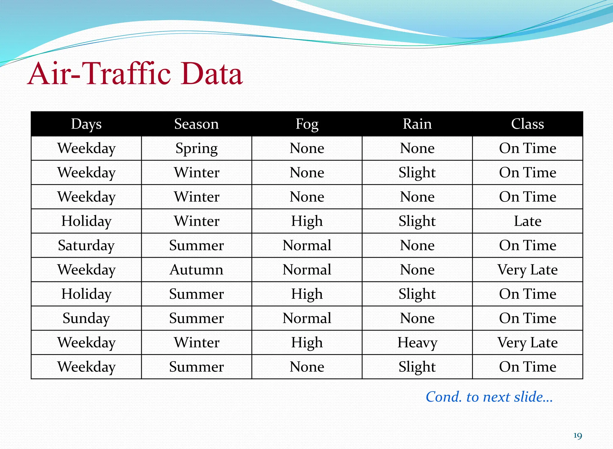
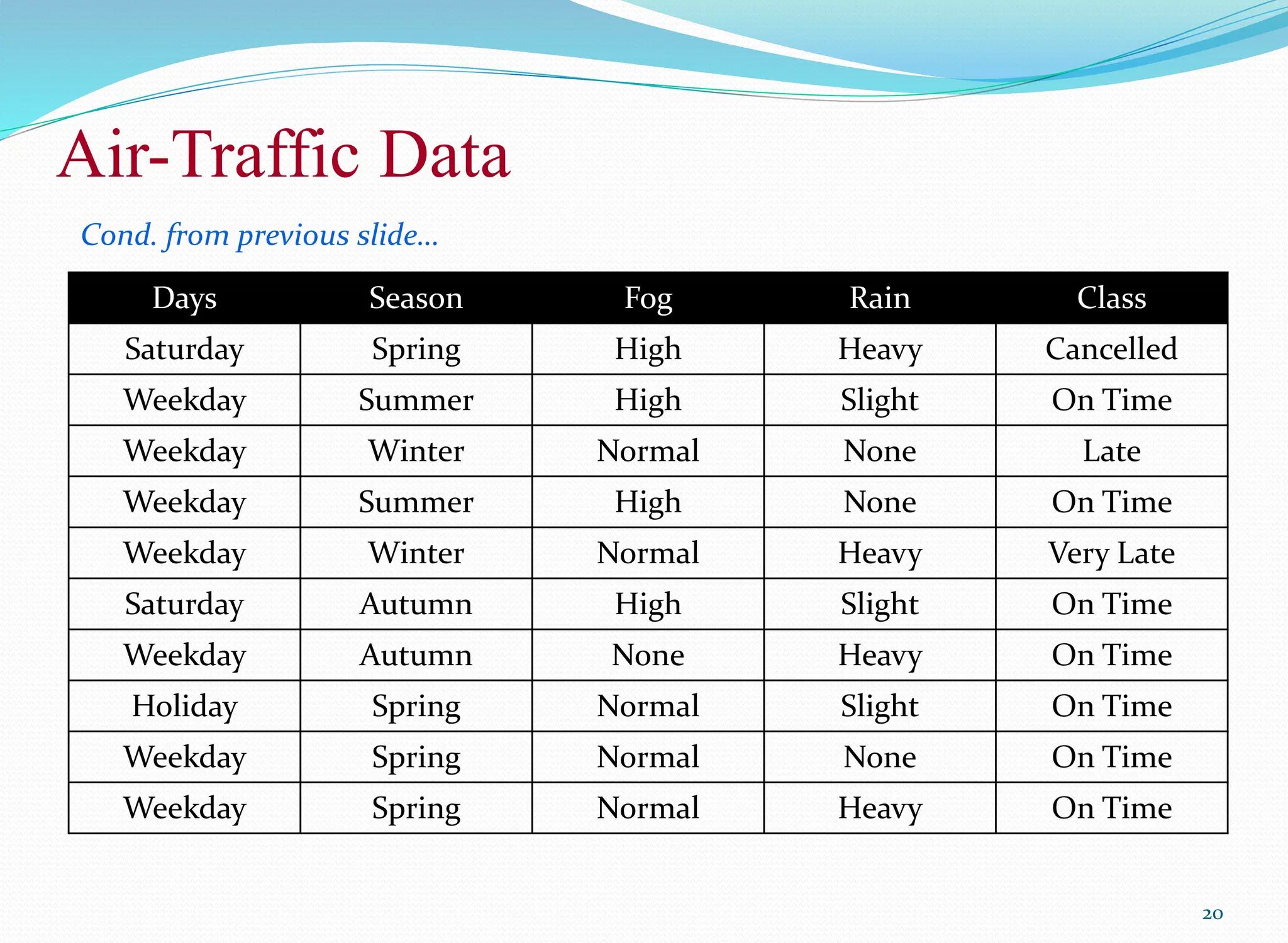
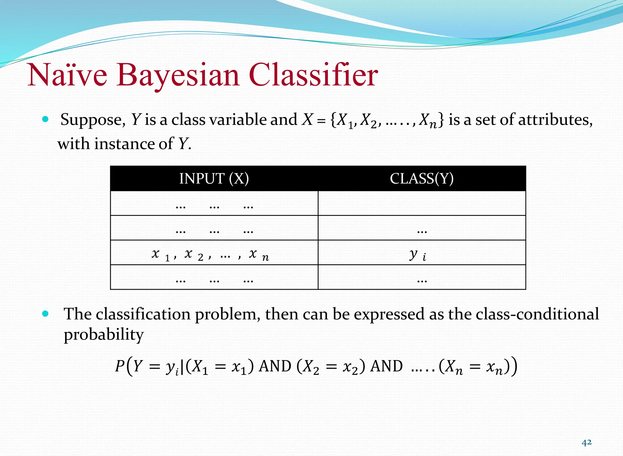
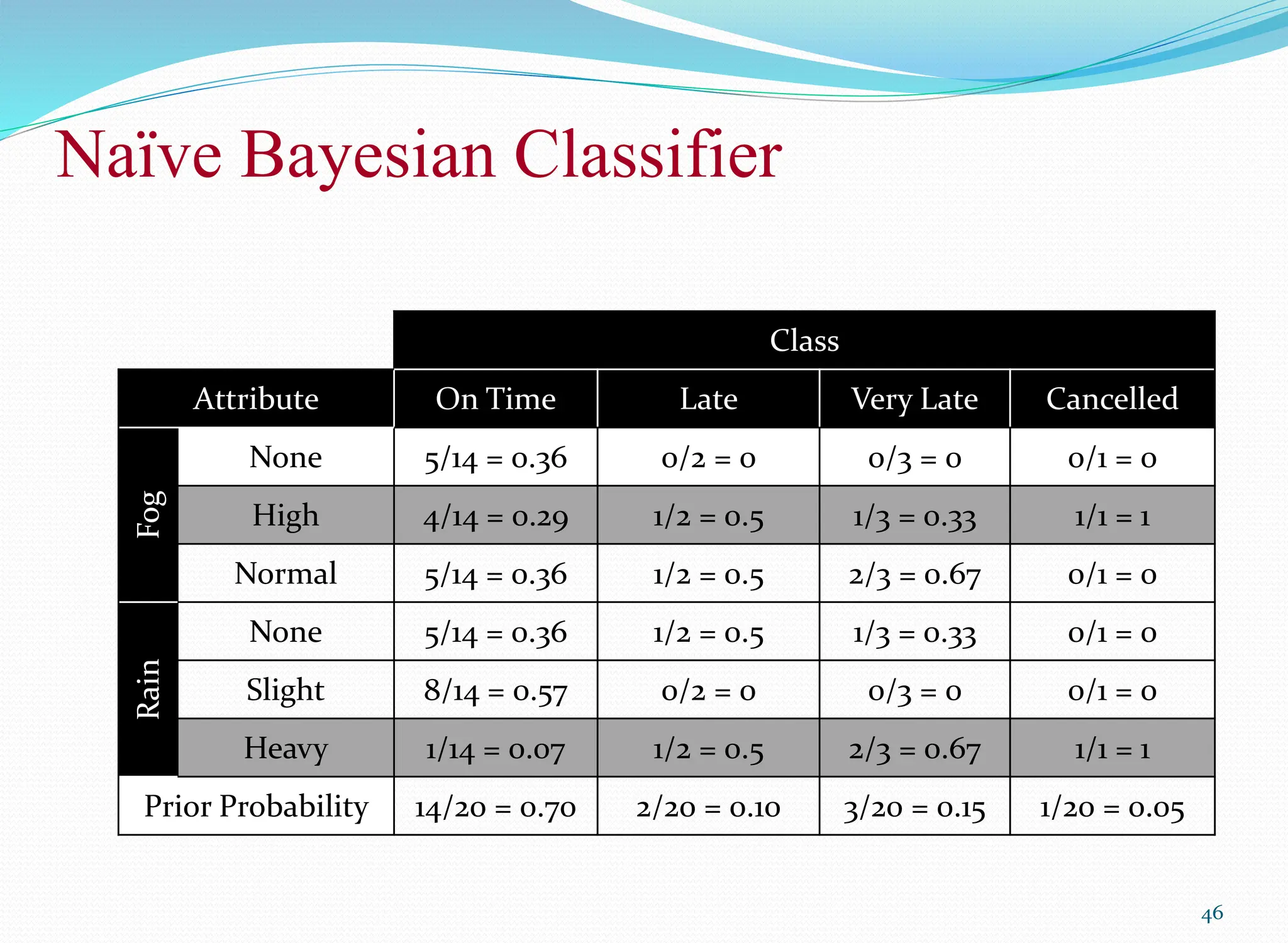
 In this database, there are four attributes
A = [ Day, Season, Fog, Rain]
with 20 tuples.
 The categories of classes are:
C= [On Time, Late, Very Late, Cancelled]
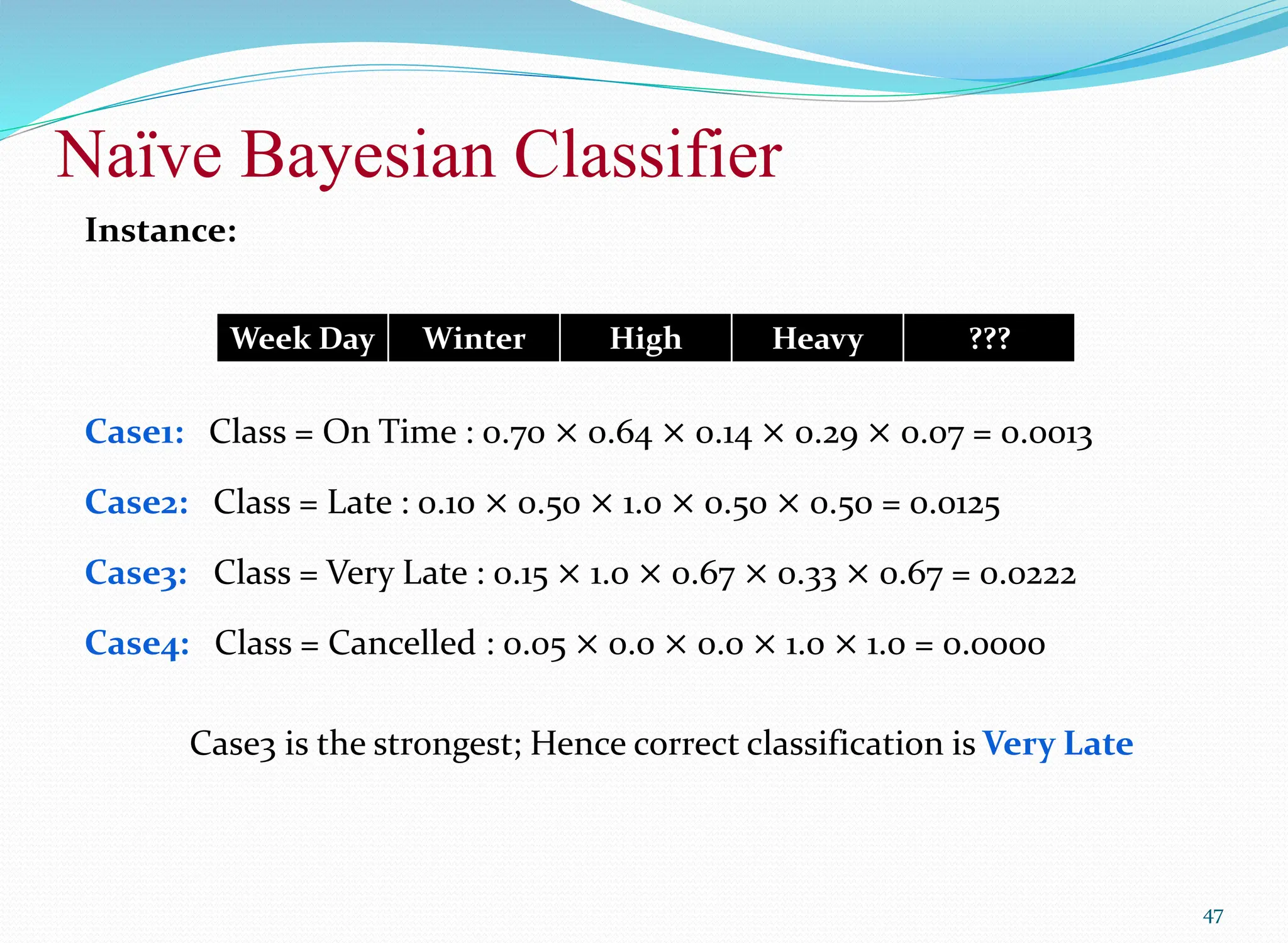
 Given this is the knowledge of data and classes, we are to find most likely
classification for any other unseen instance, for example:
 Classification technique eventually to map this tuple into an accurate class.
Week Day Winter High None ???

22. Bayesian Classifier
22
 In many applications, the relationship between the attributes set and the
class variable is non-deterministic.
 In other words, a test cannot be classified to a class label with certainty.
 In such a situation, the classification can be achieved probabilistically.
 The Bayesian classifier is an approach for modelling probabilistic
relationships between the attribute set and the class variable.
 More precisely, Bayesian classifier use Bayes’ Theorem of Probability for
classification.
 Before going to discuss the Bayesian classifier, we should have a quick look
at the Theory of Probability and then Bayes’ Theorem.

23. Bayes’ Theorem of Probability
23

24. Simple Probability
24
If there are n elementary events associated with a random experiment and m of n
of them are favorable to an event A, then the probability of happening or
occurrence of A is
𝑃 𝐴 =
𝑚
𝑛
Definition 8.2: Simple Probability

25. Simple Probability
25
 Suppose, A and B are any two events and P(A), P(B) denote the
probabilities that the events A and B will occur, respectively.
 Mutually Exclusive Events:
 Two events are mutually exclusive, if the occurrence of one precludes the
occurrence of the other OR they are separate and very different from each
other, so that it is impossible for them to exist or happen together.
Example: Tossing a coin (two events)
Tossing a ludo cube (Six events)
Can you give an example, so that two events are not mutually exclusive?
Hint: Tossing two identical coins, Weather (sunny, foggy, warm)

26. Simple Probability
26
 Independent events: Two events are independent if occurrences of one
does not alter the occurrence of other.
Example: Tossing both coin and ludo cube together.
(How many events are here?)
Can you give an example, where an event is dependent on one or more
other events(s)?
Hint: Receiving a message (A) through a communication channel (B)
over a computer (C), rain and dating.

27. Joint Probability
27
If P(A) and P(B) are the probability of two events, then
𝑃 𝐴 ∪ 𝐵 = 𝑃 𝐴 + 𝑃 𝐵 − 𝑃 𝐴 ∩ 𝐵
If A and B are mutually exclusive, then 𝑃 𝐴 ∩ 𝐵 = 0
If A and B are independent events, then 𝑃 𝐴 ∩ 𝐵 = 𝑃 𝐴 . 𝑃(𝐵)
Thus, for mutually exclusive events
𝑃 𝐴 ∪ 𝐵 = 𝑃 𝐴 + 𝑃 𝐵
Definition 8.3: Joint Probability

28. Conditional Probability
 Conditional probability as the name suggests, comes into
play when the probability of occurrence of a particular event
changes when one or more conditions are satisfied (these
conditions again are events).
 Speaking in technical terms, if X and Y are two events then
the conditional probability of X w.r.t Y is denoted by P(X|Y).
So when we talk in terms of conditional probability, just for
an example, we make a statement like "The probability of
event X given that Y has already occurred".
28

29. What if X and Y are independent events?
 From the definition of independent events, the
occurrence of event X is not dependent on event Y.
Therefore P(X|Y)=P(X).
29

30. What if X and Y are mutually exclusive?
 As X and Y are disjoint events, the probability that X will
occurs when Y has already occurred is 0.
Therefore, P(X|Y)=0.
30

31. Conditional Probability
31
If events are dependent, then their probability is expressed by conditional
probability. The probability that A occurs given that Bis denoted by 𝑃(𝐴|𝐵).
Suppose, A and B are two events associated with a random experiment. The
probability of A under the condition that B has already occurred and 𝑃(𝐵) ≠ 0 is
given by
𝑃 𝐴 𝐵 =
Number of events in 𝐵 which are favourable to 𝐴
Number of events in 𝐵
=
Number of events favourable to 𝐴 ∩ 𝐵
Number of events favourable to 𝐵
=
𝑃(𝐴 ∩ 𝐵)
𝑃(𝐵)
Definition 8.2: Conditional Probability

32. Conditional Probability
32
𝑃 𝐴 ∩ 𝐵 = 𝑃 𝐴 . 𝑃 𝐵 𝐴 , 𝑖𝑓 𝑃 𝐴 ≠ 0
or 𝑃 𝐴 ∩ 𝐵 = 𝑃 𝐵 . 𝑃 𝐴 𝐵 , 𝑖𝑓 𝑃(𝐵) ≠ 0
For three events A, B and C
𝑃 𝐴 ∩ 𝐵 ∩ 𝐶 = 𝑃 𝐴 . 𝑃 𝐵 . 𝑃 𝐶 𝐴 ∩ 𝐵
For n events A1, A2, …, An and if all events are mutually independent to each other
𝑃 𝐴1 ∩ 𝐴2 ∩ … … … … ∩ 𝐴𝑛 = 𝑃 𝐴1 . 𝑃 𝐴2 … … … … 𝑃 𝐴𝑛
Note:
𝑃 𝐴 𝐵 = 0if events are mutually exclusive
𝑃 𝐴 𝐵 = 𝑃 𝐴 if A and B are independent
𝑃 𝐴 𝐵 ⋅ 𝑃 𝐵 = 𝑃 𝐵 𝐴 ⋅ 𝑃(𝐴)otherwise,
P A ∩ B = P(B ∩ A)
Corollary 8.1: Conditional Probability

33. Conditional Probability
33
 Generalization of Conditional Probability:
P A B =
P(A ∩ B)
P(B)
=
P(B ∩ A)
P(B)
=
P(B|A)∙P(A)
P(B)
∵ P A ∩ B = P(B|A) ∙P(A) = P(A|B) ∙P(B)
By the law of total probability : P(B) = P B ∩ A ∪ B ∩ A , where A denotes
the compliment of event A. Thus,
P A B =
P(B|A) ∙ P(A)
P B ∩ A ∪ B ∩ A
=
P B A ∙ P(A)
P B A ∙ P A + P(B│A) ∙ P(A)

34. Conditional Probability
34
In general,
P A D =
P(A) ∙ P D A
P A ∙ P D A + P B ∙ P D B + P(C) ∙ P(D│C)

35. 35
Total Probability
35
Let 𝐸1, 𝐸2, … … 𝐸𝑛 be n mutually exclusive and exhaustive events associated with a
random experiment. If A is any event which occurs with 𝐸1 𝑜𝑟 𝐸2 𝑜𝑟 … … 𝐸𝑛 , then
𝑃 𝐴 = 𝑃 𝐸1 . 𝑃 𝐴 𝐸1 + 𝑃 𝐸2 . 𝑃 𝐴 𝐸2 + ⋯ … … … . +𝑃 𝐸𝑛 . 𝑃(𝐴|𝐸𝑛)
Definition 8.3: Total Probability

36. Example8.3
A bag contains 4 red and 3 black balls. A second bag contains 2 red and 4 black balls.
One bag is selected at random. From the selected bag, one ball is drawn. What is the
probability that the ball drawn is red?
This problem can be answered using the concept of Total Probability
𝐸1 =Selecting bag I
𝐸2 =Selecting bag II
A = Drawing the red ball
Thus, 𝑃 𝐴 = 𝑃 𝐸1 . 𝑃 𝐴|𝐸1 + 𝑃 𝐸2 . 𝑃(𝐴|𝐸2)
where, 𝑃 𝐴|𝐸1 = Probability of drawing red ball when first bag has been chosen
and 𝑃 𝐴|𝐸2 = Probability of drawing red ball when second bag has been chosen
36
Total Probability: An Example

37. Example 8.3:
A bag (Bag I) contains 4 red and 3 black balls. A second bag (Bag II) contains 2 red and 4
black balls. You have chosen one ball at random. It is found as red ball. What is the
probability that the ball is chosen from Bag I?
Here,
𝐸1 = Selecting bag I
𝐸2 = Selecting bag II
A = Drawing the red ball
We are to determine P(𝐸1|A). Such a problem can be solved using Bayes' theorem of
probability.
37
Reverse Probability

38. What is Bayes’ Theorem
 Bayes’ theorem is a way to figure out conditional probability.
Conditional probability is the probability of an event happening,
given that it has some relationship to one or more other events.
For example, your probability of getting a parking space is
connected to the time of day you park, where you park, and what
conventions are going on at any time.
 Bayes’ Theorem is a way of finding a probability when we know
certain other probabilities.
The formula is: P(A|B) = P(A) P(B|A)P(B)
Which tells us: how often A happens given that B happens,
written P(A|B),When we know: how often B happens given that A
happens, written P(B|A) and how likely A is on its own,
written P(A) and how likely B is on its own, written P(B)
38

39. Bayes’ Theorem
39
Let 𝐸1, 𝐸2, … … 𝐸𝑛 be n mutually exclusive and exhaustive events associated with a
random experiment. If A is any event which occurs with 𝐸1 𝑜𝑟 𝐸2 𝑜𝑟 … … 𝐸𝑛 , then
𝑃(𝐸𝑖 𝐴 =
𝑃 𝐸𝑖 . 𝑃(𝐴|𝐸𝑖)
𝑖=1
𝑛
𝑃 𝐸𝑖 . 𝑃(𝐴|𝐸𝑖)
Theorem 8.4: Bayes’Theorem

40. Example of Bayes’ Theorem
 You might wish to find a person's probability of having rheumatoid arthritis if
they have hay fever. In this example, "having hay fever" is the test for rheumatoid
arthritis (the event).
 A would be the event "patient has rheumatoid arthritis." Data indicates 10
percent of patients in a clinic have this type of arthritis. P(A) = 0.10
 B is the test "patient has hay fever." Data indicates 5 percent of patients in a clinic
have hay fever. P(B) = 0.05
 The clinic's records also show that of the patients with rheumatoid arthritis, 7
percent have hay fever. In other words, the probability that a patient has hay
fever, given they have rheumatoid arthritis, is 7 percent. B ∣ A =0.07
 Plugging these values into the theorem:
 P(A ∣ B) = (0.07 * 0.10) / (0.05) = 0.14
 So, if a patient has hay fever, their chance of having rheumatoid arthritis is 14
percent. It's unlikely a random patient with hay fever has rheumatoid arthritis.
 ss
40

41. Prior and Posterior Probabilities
41
 P(A) and P(B) are called prior probabilities
 P(A|B), P(B|A) are called posterior probabilities
Example 8.6:Prior versus Posterior Probabilities
 This table shows that the event Y has two outcomes
namely A and B, which is dependent on another event X
with various outcomes like 𝑥1, 𝑥2 and 𝑥3.
 Case1: Suppose, we don’t have any information of the
event A. Then, from the given sample space, we can
calculate P(Y = A) =
5
10
= 0.5
 Case2: Now, suppose, we want to calculate P(X =
𝑥2|Y =A) =
2
5
= 0.4 .
The later is the conditional or posterior probability, where
as the former is the prior probability.
X Y
𝑥1 A
𝑥2 A
𝑥3 B
𝑥3 A
𝑥2 B
𝑥1 A
𝑥1 B
𝑥3 B
𝑥2 B
𝑥2 A

42. Naïve Bayesian Classifier
42
 Suppose, Y is a class variable and X = 𝑋1, 𝑋2, … . . , 𝑋𝑛 is a set of attributes,
with instance of Y.
 The classification problem, then can be expressed as the class-conditional
probability
𝑃 𝑌 = 𝑦𝑖| 𝑋1 = 𝑥1 AND 𝑋2 = 𝑥2 AND … . . 𝑋𝑛 = 𝑥𝑛
INPUT (X) CLASS(Y)
… … …
… … … …
𝑥 1 , 𝑥 2 , … , 𝑥 𝑛 𝑦 𝑖
… … … …

43. Naïve Bayesian Classifier
43
 Naïve Bayesian classifier calculate this posterior probability using Bayes’
theorem, which is as follows.
 From Bayes’ theorem on conditional probability, we have
𝑃 𝑌 𝑋 =
𝑃(𝑋|𝑌) ∙ 𝑃(𝑌)
𝑃(𝑋)
=
𝑃(𝑋|𝑌) ∙ 𝑃(𝑌)
𝑃 𝑋 𝑌 = 𝑦1 ∙ 𝑃 𝑌 = 𝑦1 + ⋯ + 𝑃 𝑋 𝑌 = 𝑦𝑘 ∙ 𝑃 𝑌 = 𝑦𝑘
where,
𝑃 𝑋 = 𝑖=1
𝑘
𝑃(𝑋|𝑌 = 𝑦𝑖) ∙ 𝑃(Y = 𝑦𝑖)
Note:
 𝑃 𝑋 is called the evidence (also the total probability) and it is a constant.
 The probability P(Y|X) (also called class conditional probability) is therefore
proportional to P(X|Y)∙ 𝑃(𝑌).
 Thus, P(Y|X) can be taken as a measure of Y given that X.
P(Y|X) ≈ 𝑃 𝑋 𝑌 ∙ 𝑃(𝑌)

44. Naïve Bayesian Classifier
44
 Suppose, for a given instance of X (say x = (𝑋1 = 𝑥1) and ….. (𝑋𝑛= 𝑥𝑛)).
 There are any two class conditional probabilities namely P(Y= 𝑦𝑖|X=x)
and P(Y= 𝑦𝑗 | X=x).
 If P(Y= 𝑦𝑖 | X=x) >P(Y= 𝑦𝑗 | X=x), then we say that 𝑦𝑖 is more stronger
than 𝑦𝑗 for the instance X = x.
 The strongest 𝑦𝑖 is the classification for the instance X = x.

45. Naïve Bayesian Classifier
45
 Example: With reference to the Air Traffic Dataset mentioned earlier, let
us tabulate all the posterior and prior probabilities as shown below.
Class
Attribute On Time Late Very Late Cancelled
Day
Weekday 9/14 = 0.64 ½ = 0.5 3/3 = 1 0/1 = 0
Saturday 2/14 = 0.14 ½ = 0.5 0/3 = 0 1/1 = 1
Sunday 1/14 = 0.07 0/2 = 0 0/3 = 0 0/1 = 0
Holiday 2/14 = 0.14 0/2 = 0 0/3 = 0 0/1 = 0
Season
Spring 4/14 = 0.29 0/2 = 0 0/3 = 0 0/1 = 0
Summer 6/14 = 0.43 0/2 = 0 0/3 = 0 0/1 = 0
Autumn 2/14 = 0.14 0/2 = 0 1/3= 0.33 0/1 = 0
Winter 2/14 = 0.14 2/2 = 1 2/3 = 0.67 0/1 = 0

46. Naïve Bayesian Classifier
46
Class
Attribute On Time Late Very Late Cancelled
Fog
None 5/14 = 0.36 0/2 = 0 0/3 = 0 0/1 = 0
High 4/14 = 0.29 1/2 = 0.5 1/3 = 0.33 1/1 = 1
Normal 5/14 = 0.36 1/2 = 0.5 2/3 = 0.67 0/1 = 0
Rain
None 5/14 = 0.36 1/2 = 0.5 1/3 = 0.33 0/1 = 0
Slight 8/14 = 0.57 0/2 = 0 0/3 = 0 0/1 = 0
Heavy 1/14 = 0.07 1/2 = 0.5 2/3 = 0.67 1/1 = 1
Prior Probability 14/20 = 0.70 2/20 = 0.10 3/20 = 0.15 1/20 = 0.05

47. Naïve Bayesian Classifier
47
Instance:
Case1: Class = On Time : 0.70 × 0.64 × 0.14 × 0.29 × 0.07 = 0.0013
Case2: Class = Late : 0.10 × 0.50 × 1.0 × 0.50 × 0.50 = 0.0125
Case3: Class = Very Late : 0.15 × 1.0 × 0.67 × 0.33 × 0.67 = 0.0222
Case4: Class = Cancelled : 0.05 × 0.0 × 0.0 × 1.0 × 1.0 = 0.0000
Case3 is the strongest; Hence correct classification is Very Late
Week Day Winter High Heavy ???

48. Naïve Bayesian Classifier
CS 40003: Data Analytics 48
Note: 𝒑𝒊 ≠ 𝟏, because they are not probabilities rather proportion values (to
posterior probabilities)
Input: Given a set of k mutually exclusive and exhaustive classes C =
𝑐1, 𝑐2, … . . , 𝑐𝑘 , which have prior probabilities P(C1),P(C2),…..P(Ck).
There are n-attribute set A = 𝐴1, 𝐴2, … . . , 𝐴𝑛 , which for a given instance have
values 𝐴1 = 𝑎1,𝐴2 = 𝑎2,…..,𝐴𝑛 = 𝑎𝑛
Step: For each 𝑐𝑖 ∈ C,calculate the class condition probabilities, i = 1,2,…..,k
𝑝𝑖 = 𝑃 𝐶𝑖 ×
𝑗=1
𝑛
𝑃(𝐴𝑗 = 𝑎𝑗|𝐶𝑖)
𝑝𝑥 = max 𝑝1, 𝑝2, … . . , 𝑝𝑘
Output: 𝐶𝑥 is the classification
Algorithm: Naïve Bayesian Classification

49. Naïve Bayesian Classifier
49
Pros and Cons
 The Naïve Bayes’ approach is a very popular one, which often works well.
 However, it has a number of potential problems
 It relies on all attributes being categorical.
 If the data is less, then it estimates poorly.