Module 4 - Linear Model for Classification.pptx

BITS Pilani
Pilani Campus
BITS Pilani
Pilani Campus
Machine Learning
AIML CZG565
Linear Models for Classification
Dr. Sugata Ghosal
sugata.ghosal@pilani.bits-pilani.ac.in

BITS Pilani, Pilani Campus
• Discriminant Functions
• Probabilistic Generative Classifiers
• Probabilistic Discriminative Classifiers
• Logistic Regression
• Applications : Text classification model, Image classification
Agenda

BITS Pilani
Decision Theory
&
Classification Models

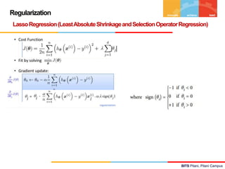
Inductive Learning Hypothesis :Interpretation
• Target Concept : t
• Discrete : f(x) ∈ {Yes, No, Maybe}
• Continuous : f(x) ∈ [20-100]
• Probability Estimation : f(x) ∈ [0-1]
5
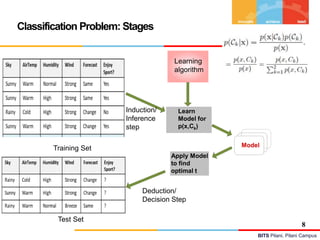
Classification
Regression

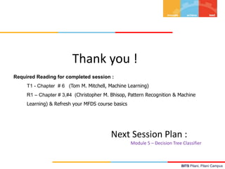
Decision Theory
• Discrete : f(x) ∈ {Yes, No} ie., t ∈ {0, 1}
6
Binary Classification

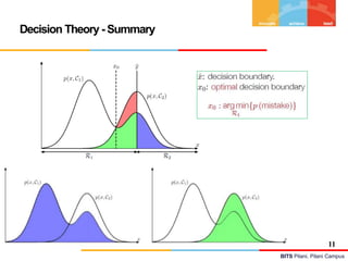
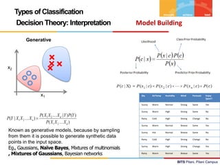
Decision Theory :
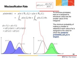
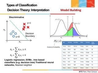
The decision problem: given x, predict t according to a probabilistic model p(x, t)
• Discrete : f(x) ∈ {Yes, No} ie., t ∈ {0, 1}
7
X =< , , , , , >  = P(Ck| X)
p(x, Ck ) is the (central!) inference problem

Classification Problem: Stages
8
Induction/
Inference
step
Deduction/
Decision Step
Test Set
Training Set Model
Learning
algorithm
Learn
Model for
p(x,Ck)
Apply Model
to find
optimal t

Decision Region
9
Induction/
Inference
step
Training Set Model
Learning
algorithm
Learn
Model for
p(x,Ck)
Model divides the input
space into regions Rk called
decision regions, one for
each class, such that all
points in Rk are assigned to
class Ck
A mistake occurs when an
input vector belonging to
class C1 is assigned to class
C2

Misclassification Rate
10
To minimize p(mistake),
each x is assigned to
whichever class has the
smaller value of the
integrand
The minimum probability of
making a mistake is
obtained if each value of x is
assigned to the class for
which the posterior
probability p(Ck|x) is
largest.

Decision Theory - Summary
11

BITS Pilani
Linear Models for Classification

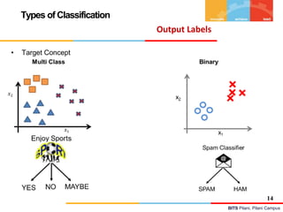
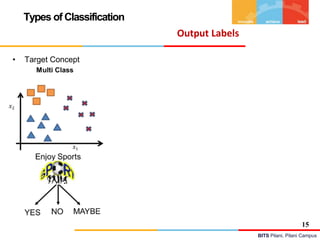
Types of Classification
Inductive Learning Hypothesis :Interpretation
• Target Concept
• Discrete : f(x) ∈ {Yes, No, Maybe}
13
Classification
Regression

Output Labels
• Target Concept
14

Output Labels
• Target Concept
15

Prediction – Multi class Classification
One Vs All Strategy(one-vs-rest)
𝑥2
𝑥1
Class 1:
Class 2:
Class 3:
ℎ𝜃
𝑖
𝑥 = 𝑃 𝑦 = 𝑖 𝑥; 𝜃 (𝑖 = 1, 2, 3)
𝑥2
𝑥1
𝑥2
𝑥1
𝑥2
𝑥1
ℎ𝜃
1
𝑥
ℎ𝜃
2
𝑥
ℎ𝜃
3
𝑥
For input x Predict ∶ max
i
ℎ𝜃
𝑖
𝑥
Note: Scikit-Learn detects when you try to use a binary classification
algorithm for a multi‐class classification task, and it automatically runs
OvA (except for SVM classifiers for which it uses OvO)

Prediction – Multi class Classification
One Vs One Strategy
𝑥2
𝑥1
Class 1:
Class 2:
Class 3:
ℎ𝜃
𝑖
𝑥 = 𝑃 𝑦 = 𝑖 𝑥; 𝜃 (𝑖 = 1, 2, 3)
ℎ𝜃
1
𝑥
ℎ𝜃
2
𝑥
ℎ𝜃
3
𝑥
For input x Predict ∶ max
i
ℎ𝜃
𝑖
𝑥
N × (N – 1) / 2 classifiers
𝑥2
𝑥1
𝑥2
𝑥1
𝑥2
𝑥1

Sky AirTemp Humidity Wind Forecast Enjoy
Sport?
Sunny Warm Normal Strong Same Yes
Sunny Warm High Strong Same No
Rainy Cold High Strong Change No
Sunny Warm Normal Breeze Same Yes
Sunny Hot Normal Breeze Same No
Sunny Warm High Strong Change Yes
Rainy Warm Normal Breeze Same Yes
Decision Theory: Interpretation Model Building
x1
x2
Generative
)
(
)
(
)
|
(
)
|
(
2
1
2
1
2
1
d
d
n
X
X
X
P
Y
P
Y
X
X
X
P
X
X
X
Y
P


 
Known as generative models, because by sampling
from them it is possible to generate synthetic data
points in the input space.
Eg., Gaussians, Naïve Bayes, Mixtures of multinomials
, Mixtures of Gaussians, Bayesian networks

Sport?
Logistic regression, SVMs , tree based
classifiers (e.g. decision tree) Traditional neural
networks, Nearest neighbor
x1
x2
Decision
Boundary
Discriminative
y=1
y=0
𝜃0 +
𝑖
𝜃𝑖𝑥𝑖 ≥ 0
𝜃0 +
𝑖
𝜃𝑖𝑥𝑖 < 0

Sport?
Logistic regression, SVMs , tree based
classifiers (e.g. decision tree) Traditional neural
networks, Nearest neighbor
𝐼𝐹 𝑂𝑈𝑇𝐿𝑂𝑂𝐾 = Overcast THEN PLAY = Yes
ELSE
𝐼𝐹 𝑂𝑈𝑇𝐿𝑂𝑂𝐾 = Rain AND WIND = Strong
THEN PLAY = No

BITS Pilani
Logistic Regression

If
If
, predict “y = 1”
, predict “y = 0”
Malignant
?
(Yes) 1
(No) 0
• Tumor Size
• Can we solve the problem using linear
regression? E.g., fit a straight line and
define a threshold at 0.5
• Threshold classifier output h(x) at 0.5:
Logistic Regression vs Least Squares Regression
A Discriminant function f (x)
directly map input to class labels
In two-class problem, f (.) is binary valued

Decision Rules
• Classifier:
f (x,w) = wo + wT x (linear discriminant function)
• Decision rule is
• Mathematically
y = sign(w0 + wT x)
• This specifies a linear classifier: it has a linear boundary (hyperplane)
w0 + wT x = 0
A discriminant is a function that takes an input vector x and assigns it
to one of K classes, denoted Ck.

Learning model parameters
• Training set:
• m examples
• How to choose parameters (feature weights) ?
27

Logistic Regression
• ℎ𝜃 𝑥 = 𝑔 𝜃0 + 𝜃1𝑥1 + 𝜃2𝑥2
– e.g., 𝜃0 = −3, 𝜃1 = 1, 𝜃2 = 1
• Predict “𝑦 = 1” if −3 + 𝑥1 + 𝑥2 ≥ 0
• At decision boundary output of logistic regression is 0.5
Tumor Size
Age
Decision
boundary
Slide credit: Andrew Ng

Logistic Regression
Slide credit: Andrew Ng

Logistic Regression
• Training set:
• How to choose parameters (feature weights)?
• m examples
• n features

Logistic Regression
• Training set:
• How to choose parameters (feature weights)?
“non-convex” “convex”

Logistic regression cost function (cross entropy)
If y = 1
1
0
Cost

Logistic regression cost function
If y = 0
1
0
Cost
Cost=0; If y=0 and hꝊ(x)=0

Output :
To fit parameters : Apply Gradient Descent Algorithm
To make a prediction given new :
Cost function

Gradient Descent Algorithm
𝐽 𝜃 = −
1
𝑚
𝑖=1
𝑚
𝑦(𝑖)
log ℎ𝜃 𝑥(𝑖)
+ (1 − 𝑦(𝑖)
) log 1 − ℎ𝜃 𝑥(𝑖)
Goal: min
𝜃
𝐽(𝜃)
Repeat
{
𝜃𝑗 ≔ 𝜃𝑗 − 𝛼
𝜕
𝜕𝜃𝑗
𝐽 𝜃
}
𝜕
𝜕𝜃𝑗
𝐽 𝜃 =
1
𝑚
𝑖=1
𝑚
(ℎ𝜃 𝑥 𝑖
− 𝑦(𝑖)
) 𝑥𝑗
(𝑖)

Linear Regression
Repeat {
1
𝑚
𝑖=1
𝑚
ℎ𝜃 𝑥 𝑖
− 𝑦(𝑖)
𝑥𝑗
(𝑖)
}
Logistic Regression
Repeat {
1
𝑚
𝑖=1
𝑚
ℎ𝜃 𝑥 𝑖
− 𝑦(𝑖)
𝑥𝑗
(𝑖)
}
ℎ𝜃 𝑥 = 𝜃⊤
𝑥
ℎ𝜃 𝑥 =
1
1 + 𝑒−𝜃⊤𝑥
Slide credit: Andrew
Ng
Gradient Descent Algorithm

Example: Sentiment Analysis
Sentiment Features

Classifying sentiment using logistic regression

Logistic Regression – Fit a Model
CGPA IQ IQ Job Offered
5.5 6.7 100 1
5 7 105 0
8 6 90 1
9 7 105 1
6 8 120 0
7.5 7.3 110 0
Hyper parameters:
Learning Rate = 0.3
Initial Weights = (0.5, 0.5,0.5)
Regularization Constant = 0
𝜃TX = 0.5 +0.5 CGPA + 0.5 IQ
ℎ𝜃 𝑥 =
1
1 + 𝑒−𝜃⊤𝑥
𝜃𝐶𝐺𝑃𝐴 ≔ 𝜃𝐶𝐺𝑃𝐴 − 0.3
1
6
𝑖=1
6
ℎ𝜃 𝑥 𝑖
− 𝑦(𝑖)
𝑥𝐶𝐺𝑃𝐴
(𝑖)
𝜃𝐼𝑄 ≔ 𝜃𝐼𝑄 − 0.3
1
6
𝑖=1
6
ℎ𝜃 𝑥 𝑖
− 𝑦(𝑖)
𝑥𝐼𝑄
(𝑖)
𝜃0 ≔ 𝜃0 − 0.3
1
6
𝑖=1
6
ℎ𝜃 𝑥 𝑖
− 𝑦 𝑖
(1)
ℎ𝜃 𝑥 =
1
1 + 𝑒−(0.5 +0.5 𝐶𝐺𝑃𝐴 + 0.5 𝐼𝑄 )
Approx. : New weights
𝜃0 = 0.4
𝜃1=𝐶𝐺𝑃𝐴 =-0.4
𝜃2=𝐼𝑄 = −0.6

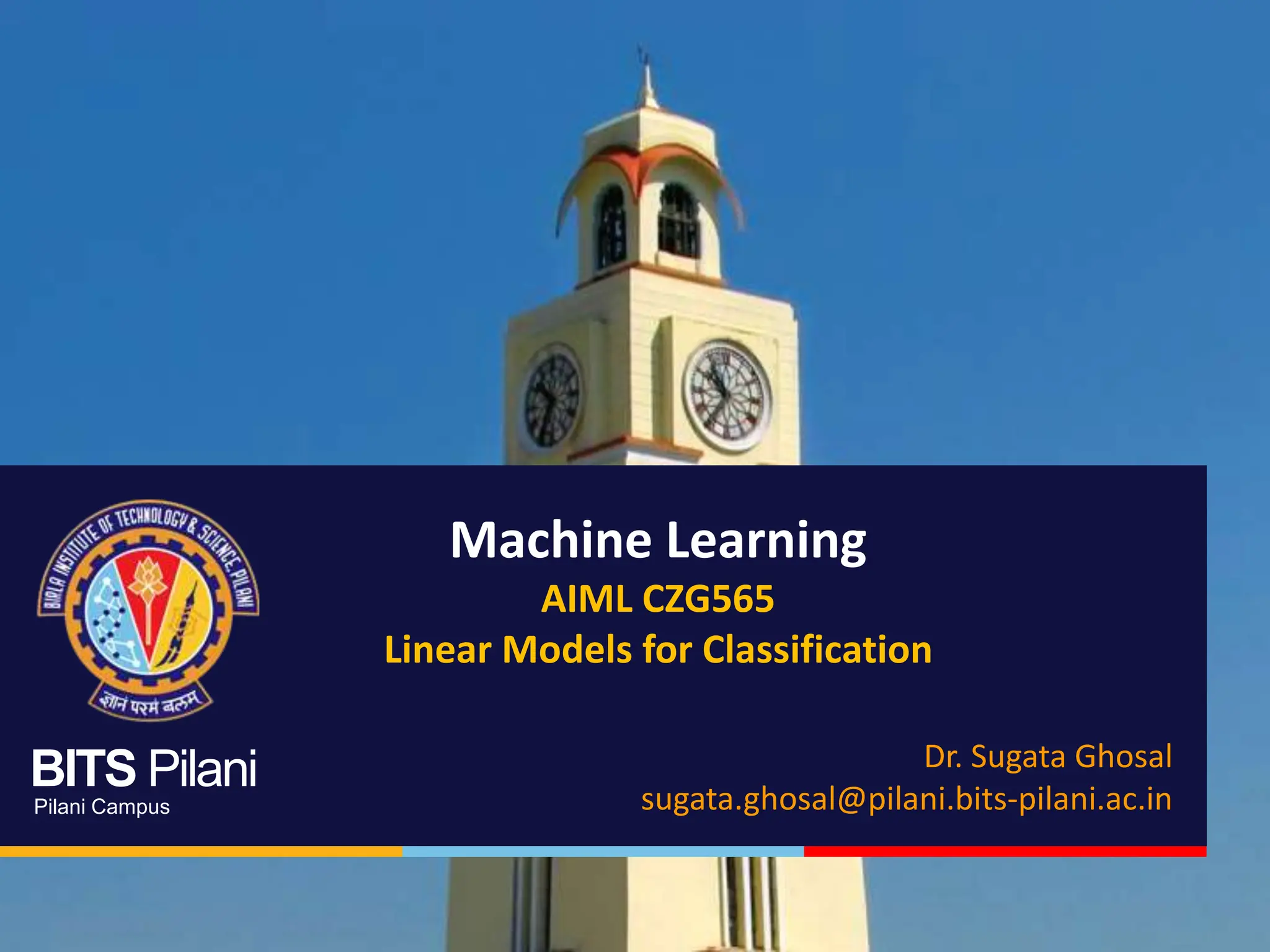
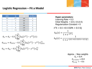
Logistic Regression – Inference & Interpretation
CGPA IQ IQ Job Offered
5.5 6.7 100 1
5 7 105 0
8 6 90 1
9 7 105 1
6 8 120 0
7.5 7.3 110 0
Assume : 0.4+0.3CGPA-0.45IQ
Predict the Job offered for a candidate : (5, 6)
h(x) = 0.31
Y-Predicted = 0 / No
Note :
The exponential function of the regression coefficient (ew-cpga) is the odds ratio associated with a one-unit
increase in the cgpa.
+ The odd of being offered with job increase by a factor of 1.35 for every unit increase in the CGPA
[np.exp(model.params)]

Logistic regression (Classification)
• Model
ℎ𝜃 𝑥 = 𝑃 𝑌 = 1 𝑋1, 𝑋2, ⋯ , 𝑋𝑛 =
1
1+𝑒−𝜃⊤𝑥
• Cost function
𝐽 𝜃 =
1
𝑚
𝑖=1
𝑚
Cost(ℎ𝜃(𝑥 𝑖
), 𝑦(𝑖)
)) Cost(ℎ𝜃 𝑥 , 𝑦) =
−log ℎ𝜃 𝑥 if 𝑦 = 1
−log 1 − ℎ𝜃 𝑥 if 𝑦 = 0
• Learning
Gradient descent: Repeat {𝜃𝑗 ≔ 𝜃𝑗 − 𝛼
1
𝑚 𝑖=1
𝑚
ℎ𝜃 𝑥 𝑖
− 𝑦 𝑖
𝑥𝑗
𝑖
}
• Inference
𝑌 = ℎ𝜃 𝑥test
=
1
1 + 𝑒−𝜃⊤𝑥test
Note:
• σ(t) < 0.5 when t < 0, and σ(t) ≥ 0.5 when t ≥ 0, so a Logistic model predicts 1 if xTθ is positive, and 0 if it is negative
• logit(p) = log(p / (1 - p)), is the inverse of the logistic function. Indeed, if you compute the logit of the estimated probability
p, you will find that the result is t. The logit is also called the log-odds

Overfitting vs Underfitting
Overfitting
• Fitting the data too well
– Features are noisy / uncorrelated to
concept
Underfitting
• Learning too little of the true
concept
– Features don’t capture concept
– Too much bias in model
0
0.1
0.2
0.3
0.4
0.5
0.6
0.7
0.8
0.9
1
0 0.1 0.2 0.3 0.4 0.5 0.6 0.7 0.8 0.9 1

BITS Pilani
Regularization
Note : This topic is already covered in the module 3 . Refresher & few more
points added here

Regularization

Ways to Control Overfitting
• Regularization
𝐿𝑜𝑠𝑠 𝑆 =
𝑖
𝑛
𝐿𝑜𝑠𝑠(𝑦𝑖
^
, 𝑦𝑖) + 𝛼
𝑗
# 𝑊𝑒𝑖𝑔ℎ𝑡𝑠
|θ𝑗|
45
Note:
The hyperparameter controlling the regularization strength of a Scikit-Learn LogisticRegression model is not
alpha (as in other linear models), but its inverse: C. The higher the value of C, the less the model is
regularized.

Understanding Regularization

Regularization
RidgeRegression/Tikhonovregularization

Regularization
LassoRegression(LeastAbsoluteShrinkageandSelectionOperatorRegression)

Thank you !
Next Session Plan :
Module 5 – Decision Tree Classifier
Required Reading for completed session :
T1 - Chapter # 6 (Tom M. Mitchell, Machine Learning)
R1 – Chapter # 3,#4 (Christopher M. Bhisop, Pattern Recognition & Machine
Learning) & Refresh your MFDS course basics

Module 4 - Linear Model for Classification.pptx

Recommended

Recommended

More Related Content

Similar to Module 4 - Linear Model for Classification.pptx

Similar to Module 4 - Linear Model for Classification.pptx (20)

Recently uploaded

Recently uploaded (20)

Module 4 - Linear Model for Classification.pptx