- POSTECH EECE695J, "딥러닝 기초 및 철강공정에의 활용", Lecture 2 - Contents: categorization of machine learning, supervised learning (linear regression and logistic regression), multiclass classification

1. Supervised Learning
Sang Jun Lee
(Ph.D. candidate, POSTECH)
EECE695J 전자전기공학특론J(딥러닝기초및철강공정에의활용) – LECTURE 2 (2017. 9. 7)

2. 2
▣ 지난 시간 내용
▲ Python 코딩의 기초 및 필수 패키지 (NumPy, SciPy, Matplotlilb)
▲ TensorFlow: tensor, data flow graph, session
▲ TensorFlow 설치해 본 사람? ㅋㅋ
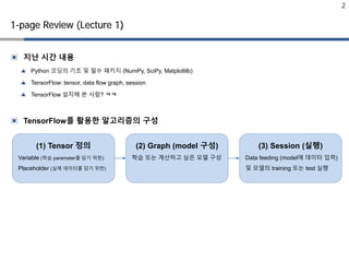
▣ TensorFlow를 활용한 알고리즘의 구성
1-page Review (Lecture 1)
(1) Tensor 정의
Variable (학습 parameter를 담기 위한)
Placeholder (실제 데이터를 담기 위한)
(2) Graph (model 구성)
학습 또는 계산하고 싶은 모델 구성
(3) Session (실행)
Data feeding (model에 데이터 입력)
및 모델의 training 또는 test 실행

3. 3
What is Machine Learning?
우리가 필요로 하는 것은:
• 모델링에 의한 혹은 규칙기반 알고리즘이 가지는 한계를 극복하기 위한 데이터 기반의 알고리즘!
• Machine learning에 어떤 기법들이 있고, 내 문제에 대한 올바른 접근 방법을 알아야..
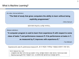
(An older, informal definition)
“The field of study that gives computers the ability to learn without being
explicitly programmed.”
- Arthur Samuel -
컴퓨터에게 학습하는 능력을 부여하는..
(Modern definition)
“A computer program is said to learn from experience E with respect to some
class of tasks T and performance measure P, if its performance at tasks in T,
as measured by P, improves with experience E.”
- Tom Mitchell -
Experience (E), task (T), performance measure (P).. 좀 더 복잡한 기계학습 기법들을 포함하기 위한 정의..

4. 4
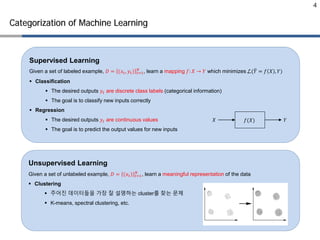
Categorization of Machine Learning
Unsupervised Learning
Given a set of unlabeled example, 𝐷𝐷 = (𝑥𝑥𝑡𝑡) 𝑡𝑡=1
𝑁𝑁
, learn a meaningful representation of the data
 Clustering
 주어진 데이터들을 가장 잘 설명하는 cluster를 찾는 문제
 K-means, spectral clustering, etc.
Supervised Learning
Given a set of labeled example, 𝐷𝐷 = (𝑥𝑥𝑡𝑡, 𝑦𝑦𝑡𝑡) 𝑡𝑡=1
𝑁𝑁
, learn a mapping 𝑓𝑓: 𝑋𝑋 → 𝑌𝑌 which minimizes L(�𝑌𝑌 = 𝑓𝑓 𝑋𝑋 , 𝑌𝑌)
 Classification
 The desired outputs 𝑦𝑦𝑡𝑡 are discrete class labels (categorical information)
 The goal is to classify new inputs correctly
 Regression
 The desired outputs 𝑦𝑦𝑡𝑡 are continuous values
 The goal is to predict the output values for new inputs
𝑓𝑓(𝑋𝑋)𝑋𝑋 𝑌𝑌

5. 5
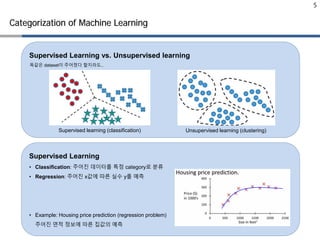
Categorization of Machine Learning
Supervised Learning vs. Unsupervised learning
Supervised learning (classification) Unsupervised learning (clustering)
Supervised Learning
• Classification: 주어진 데이터를 특정 category로 분류
• Regression: 주어진 x값에 따른 실수 y를 예측
• Example: Housing price prediction (regression problem)
주어진 면적 정보에 따른 집값의 예측
똑같은 dataset이 주어졌다 할지라도..

6. 6
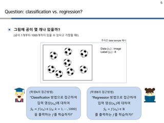
Question: classification vs. regression?
▣ 그림에 공이 몇 개나 있을까?
(공이 1개부터 1000개까지 있을 수 있다고 가정할 때!)
(학생A의 접근방법)
“Classification 방법으로 접근하여
입력 영상(𝑥𝑥𝑘𝑘)에 대하여
�𝑦𝑦𝑘𝑘 = 𝑓𝑓 𝑥𝑥𝑘𝑘 ∈ {𝑐𝑐𝑘𝑘: 𝑘𝑘 = 1, ⋯ , 1000}
을 출력하는 𝑓𝑓를 학습하자!”
(학생B의 접근방법)
“Regression 방법으로 접근하여
입력 영상(𝑥𝑥𝑘𝑘)에 대하여
�𝑦𝑦𝑘𝑘 = 𝑓𝑓 𝑥𝑥𝑘𝑘 ∈ ℝ
를 출력하는 𝑓𝑓를 학습하자!”
Data (𝑥𝑥𝑖𝑖) : image
Label (𝑦𝑦𝑖𝑖) : 8
주어진 data sample 예시

7. 8
▣ (example) Housing price prediction
▲ 면적과 화장실의 수를 고려한 집 값의 예측
▲ ℎ𝜽𝜽 𝒙𝒙 = 𝜃𝜃0 + 𝜃𝜃1 𝑥𝑥1 + 𝜃𝜃2 𝑥𝑥2
ℎ𝜽𝜽 is a hypothesis function parameterized by 𝜽𝜽
▲ Linear regression problem:
Find an optimal 𝜽𝜽∗
that minimizes 𝐽𝐽(ℎ𝜽𝜽 𝑋𝑋 , 𝑌𝑌)
▣ Ordinary least square regression model:
▲ 만약 데이터가 n-dimensional 이라면.. (𝒙𝒙 ∈ ℝ𝑛𝑛+1
, 𝑥𝑥0 = 1)
▲ Cost function: ℎ𝜽𝜽 𝒙𝒙 가 얼마나 좋은 hypothesis function인지 평가하는 measure
Linear Regression
𝑋𝑋 𝑌𝑌
ℎ𝜽𝜽 𝒙𝒙 = Σ𝑖𝑖=0
𝑛𝑛
𝜃𝜃𝑖𝑖 𝑥𝑥𝑖𝑖 = 𝜽𝜽𝑇𝑇
𝒙𝒙
𝐽𝐽 𝜽𝜽 =
1
2
Σ𝑖𝑖=1
𝑚𝑚
ℎ𝜽𝜽 𝒙𝒙 𝒊𝒊
− 𝑦𝑦 𝑖𝑖 2
EECE695J (2017)
Sang Jun Lee (POSTECH)
Squared loss

8. 9
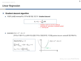
▣ Gradient descent algorithm
▲ 어떻게 𝐽𝐽 𝜽𝜽 를 minimize하는 최적 𝜽𝜽∗
를 찾을 것인가? Gradient descent
▲ (example) 𝑓𝑓 𝑥𝑥 = 𝑥𝑥2
− 2𝑥𝑥 + 3
(우리는 이 함수가 (1,2)에서 최소값을 가지는 것을 알지만.. 이것을 gradient descent method로 접근해보자!)
Linear Regression
𝜃𝜃𝑗𝑗 ≔ 𝜃𝜃𝑗𝑗 − 𝛼𝛼
𝜕𝜕
𝜕𝜕𝜃𝜃𝑗𝑗
𝐽𝐽 𝜽𝜽
Assume that 𝑥𝑥0 = 3
𝑑𝑑
𝑑𝑑𝑑𝑑
𝑓𝑓 𝑥𝑥
𝑥𝑥=𝑥𝑥0
= 2𝑥𝑥 − 2 𝑥𝑥=3 = 4
𝑥𝑥𝑖𝑖+1 ≔ 𝑥𝑥𝑖𝑖 − 𝛼𝛼
𝑑𝑑
𝑑𝑑𝑑𝑑
𝑓𝑓 𝑥𝑥
𝑥𝑥=𝑥𝑥𝑖𝑖
𝑓𝑓 𝑥𝑥 = 𝑥𝑥2
− 2𝑥𝑥 + 3
𝑦𝑦
𝑥𝑥
기울기: +
EECE695J (2017)
Sang Jun Lee (POSTECH)
• Gradient (기울기)가 감소하는 방향으로
parameter (𝜽𝜽 : optimization variable)를 update!
• 𝛼𝛼 : learning rate

9. 10
▣ Gradient descent algorithm
▲ 어떻게 𝐽𝐽 𝜽𝜽 를 minimize하는 최적 𝜽𝜽∗
를 찾을 것인가? Gradient descent
▲ Linear regression 문제로 돌아와서..
▲ Update rule: (for 𝑗𝑗 = 0, ⋯ , 𝑛𝑛, 𝑖𝑖 = 1, ⋯ , 𝑚𝑚)
Linear Regression
𝜃𝜃𝑗𝑗 ≔ 𝜃𝜃𝑗𝑗 − 𝛼𝛼
𝜕𝜕
𝜕𝜕𝜃𝜃𝑗𝑗
𝐽𝐽 𝜽𝜽
𝜕𝜕
𝜕𝜕𝜃𝜃𝑗𝑗
𝐽𝐽 𝜽𝜽 =
𝜕𝜕
𝜕𝜕𝜃𝜃𝑗𝑗
1
2
ℎ𝜽𝜽 𝒙𝒙 − 𝑦𝑦 2
= 2 ⋅
1
2
ℎ𝜽𝜽 𝒙𝒙 − 𝑦𝑦 ⋅
𝜕𝜕
𝜕𝜕𝜃𝜃𝑗𝑗
ℎ𝜽𝜽 𝒙𝒙 − 𝑦𝑦
= ℎ𝜽𝜽 𝒙𝒙 − 𝑦𝑦 ⋅
𝜕𝜕
𝜕𝜕𝜃𝜃𝑗𝑗
(Σ𝑖𝑖=0
𝑛𝑛
𝜃𝜃𝑖𝑖 𝑥𝑥𝑖𝑖 − 𝑦𝑦)
= ℎ𝜽𝜽 𝒙𝒙 − 𝑦𝑦 ⋅ 𝑥𝑥𝑗𝑗
𝜃𝜃𝑗𝑗 ≔ 𝜃𝜃𝑗𝑗 − 𝛼𝛼 ℎ𝜽𝜽 𝒙𝒙 𝑖𝑖
− 𝑦𝑦 𝑖𝑖
⋅ 𝑥𝑥𝑗𝑗
(𝑖𝑖)
EECE695J (2017)
Sang Jun Lee (POSTECH)

10. 11
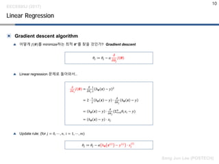
▣ Linear regression 문제를 (한 번에) 푸는 또 다른 접근 방법!
▲ 주어진 linear regression 문제 : Given 𝒙𝒙 𝒊𝒊
, 𝑦𝑦 𝑖𝑖
𝑖𝑖 = 1, ⋯ , 𝑚𝑚}, find 𝜽𝜽∗
which minimizes 𝐽𝐽(𝜽𝜽)
▲ 여기서 𝐽𝐽(𝜽𝜽)를 matrix form으로 표현하면..
, where 𝑋𝑋 =
−𝒙𝒙 𝟏𝟏 𝑇𝑇
−
⋮
−𝒙𝒙 𝒎𝒎 𝑇𝑇
−
, 𝜽𝜽 =
𝜃𝜃0
⋮
𝜃𝜃𝑛𝑛
, and 𝒚𝒚 =
𝑦𝑦(1)
⋮
𝑦𝑦(𝑚𝑚)
Normal Equation
𝐽𝐽 𝜽𝜽 =
1
2
𝑋𝑋𝜽𝜽 − 𝒚𝒚 𝑇𝑇
𝑋𝑋𝜽𝜽 − 𝒚𝒚
EECE695J (2017)
Sang Jun Lee (POSTECH)

11. 12
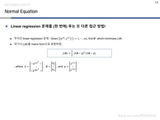
▣ 참고!
(자주 사용되는 vector derivatives)
▲ The derivative of 𝐽𝐽 with respect to 𝜽𝜽 is: vector 𝜽𝜽와 동일한 length를 가지는 column vector!
▲ 어떤 symmetric matrix 𝑃𝑃에 대하여
(역시 scalar인 𝜽𝜽𝑇𝑇
𝑃𝑃𝜽𝜽를 vector에 대하여 미분하니 column vector가 됨!)
▲ 어떤 column vector 𝒙𝒙에 대하여
Normal Equation
𝛻𝛻𝜽𝜽 𝐽𝐽 𝜽𝜽 =
𝜕𝜕𝐽𝐽(𝜽𝜽)
𝜕𝜕𝜃𝜃0
⋮
𝜕𝜕𝐽𝐽(𝜽𝜽)
𝜕𝜕𝜃𝜃𝑛𝑛
𝛻𝛻𝜽𝜽 𝜽𝜽𝑇𝑇
𝑃𝑃𝜽𝜽 = 2𝑃𝑃𝜽𝜽
𝛻𝛻𝜽𝜽 𝜽𝜽𝑇𝑇
𝒙𝒙 = 𝒙𝒙
multi-variable
single-valued function
EECE695J (2017)
Sang Jun Lee (POSTECH)

12. 13
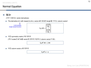
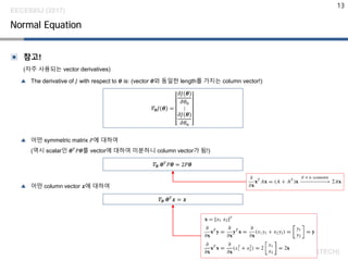
▣ 참고!
(자주 사용되는 vector derivatives)
▲ The derivative of 𝐽𝐽 with respect to 𝜽𝜽 is: (vector 𝜽𝜽와 동일한 length를 가지는 column vector!)
▲ 어떤 symmetric matrix 𝑃𝑃에 대하여
(역시 scalar인 𝜽𝜽𝑇𝑇
𝑃𝑃𝜽𝜽를 vector에 대하여 미분하니 column vector가 됨!)
▲ 어떤 column vector 𝒙𝒙에 대하여
Normal Equation
𝛻𝛻𝜽𝜽 𝐽𝐽 𝜽𝜽 =
𝜕𝜕𝐽𝐽(𝜽𝜽)
𝜕𝜕𝜃𝜃0
⋮
𝜕𝜕𝐽𝐽(𝜽𝜽)
𝜕𝜕𝜃𝜃𝑛𝑛
𝛻𝛻𝜽𝜽 𝜽𝜽𝑇𝑇
𝑃𝑃𝜽𝜽 = 2𝑃𝑃𝜽𝜽
𝛻𝛻𝜽𝜽 𝜽𝜽𝑇𝑇
𝒙𝒙 = 𝒙𝒙
EECE695J (2017)
Sang Jun Lee (POSTECH)

13. 14
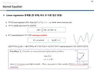
▣ Linear regression 문제를 (한 번에) 푸는 또 다른 접근 방법!
▲ 주어진 linear regression 문제 : Given 𝒙𝒙 𝒊𝒊
, 𝑦𝑦 𝑖𝑖
𝑖𝑖 = 1, ⋯ , 𝑚𝑚}, find 𝜽𝜽∗
which minimizes 𝐽𝐽(𝜽𝜽)
▲ 여기서 𝐽𝐽(𝜽𝜽)를 matrix form으로 표현하면..
▲ 𝜽𝜽∗
가 optimal solution이 되기 위한 necessary condition:
(일반적으로) 𝛻𝛻𝜽𝜽 𝐽𝐽 𝜽𝜽∗
= 0를 만족하는 𝜽𝜽∗
가 여러 개 일 수 있는데 이 모두가 optimal solution인 것은 보장되지 않지만..
Normal Equation
𝐽𝐽 𝜽𝜽 =
1
2
𝑋𝑋𝜽𝜽 − 𝒚𝒚 𝑇𝑇
𝑋𝑋𝜽𝜽 − 𝒚𝒚
𝜽𝜽∗
is an optimal → 𝛻𝛻𝜽𝜽 𝐽𝐽 𝜽𝜽∗
= 0
EECE695J (2017)
Sang Jun Lee (POSTECH)

14. 15
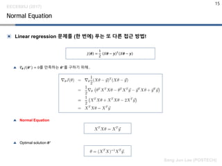
▣ Linear regression 문제를 (한 번에) 푸는 또 다른 접근 방법!
▲ 𝛻𝛻𝜽𝜽 𝐽𝐽 𝜽𝜽∗
= 0를 만족하는 𝜽𝜽∗
를 구하기 위해..
▲ Normal Equation
▲ Optimal solution 𝜽𝜽∗
Normal Equation
𝐽𝐽 𝜽𝜽 =
1
2
𝑋𝑋𝜽𝜽 − 𝒚𝒚 𝑇𝑇
𝑋𝑋𝜽𝜽 − 𝒚𝒚
EECE695J (2017)
Sang Jun Lee (POSTECH)

15. 16
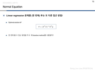
▣ Linear regression 문제를 (한 번에) 푸는 또 다른 접근 방법!
▲ Optimal solution 𝜽𝜽∗
▲ 한 번에 풀 수 있는 방법을 두고 왜 iterative method를 사용할까?
Normal Equation
EECE695J (2017)
Sang Jun Lee (POSTECH)

16. 17
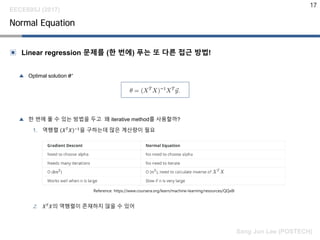
▣ Linear regression 문제를 (한 번에) 푸는 또 다른 접근 방법!
▲ Optimal solution 𝜽𝜽∗
▲ 한 번에 풀 수 있는 방법을 두고 왜 iterative method를 사용할까?
1. 역행렬 𝑋𝑋 𝑇𝑇
𝑋𝑋 −1
을 구하는데 많은 계산량이 필요
2. 𝑋𝑋 𝑇𝑇
𝑋𝑋의 역행렬이 존재하지 않을 수 있어
Normal Equation
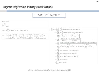
Reference: https://www.coursera.org/learn/machine-learning/resources/QQx8l
EECE695J (2017)
Sang Jun Lee (POSTECH)

17. 18
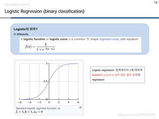
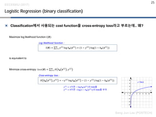
Logistic Regression (binary classification)
Logistic의 의미?
In Wikipedia,
Logistic regression: 입력데이터 𝑥𝑥에 대하여
bound (0 ≤ 𝑓𝑓 𝑥𝑥 ≤ 1)가 있는 실수 값으로
regression
EECE695J (2017)
Sang Jun Lee (POSTECH)

18. 19
▣ Logistic regression을 왜 classification 문제라고 할까?
▲ Logistic regression
▲ ℎ𝜽𝜽 𝒙𝒙 를 확률처럼 이해:
▲ Decision boundary for classification:
Logistic Regression (binary classification)
ℎ𝜽𝜽 𝒙𝒙 = 𝑃𝑃 𝑦𝑦 = 1 𝒙𝒙 ; 𝜽𝜽) = 1 − 𝑃𝑃 𝑦𝑦 = 0 𝒙𝒙 ; 𝜽𝜽)
ℎ𝜽𝜽 𝒙𝒙 =
1
1 + 𝑒𝑒−𝜽𝜽𝑇𝑇 𝒙𝒙
x 𝑔𝑔 𝒛𝒛 =
1
1 + 𝑒𝑒−𝑧𝑧
ℎ𝜽𝜽 𝒙𝒙𝒙𝒙
𝜽𝜽
𝑧𝑧
Sigmoid function
(or logistic function)
Output의 range를 0~1 사이의 값으로 제한!
ℎ𝜽𝜽 𝒙𝒙 ≥ 0.5 → 𝑦𝑦 = 1
ℎ𝜽𝜽 𝒙𝒙 < 0.5 → 𝑦𝑦 = 0
EECE695J (2017)
Sang Jun Lee (POSTECH)

19. 20
▣ Logistic regression을 왜 classification 문제라고 할까?
▲ Logistic regression
▲ ℎ𝜽𝜽 𝒙𝒙 를 확률처럼 이해:
▲ Decision boundary for classification:
Logistic Regression (binary classification)
ℎ𝜽𝜽 𝒙𝒙 = 𝑃𝑃 𝑦𝑦 = 1 𝒙𝒙 ; 𝜽𝜽) = 1 − 𝑃𝑃 𝑦𝑦 = 0 𝒙𝒙 ; 𝜽𝜽)
ℎ𝜽𝜽 𝒙𝒙 =
1
1 + 𝑒𝑒−𝜽𝜽𝑇𝑇 𝒙𝒙
x 𝑔𝑔 𝒛𝒛 =
1
1 + 𝑒𝑒−𝑧𝑧
ℎ𝜽𝜽 𝒙𝒙𝒙𝒙
𝜽𝜽
𝑧𝑧
Sigmoid function
(or logistic function)
Output의 range를 0~1 사이의 값으로 제한!
ℎ𝜽𝜽 𝒙𝒙 ≥ 0.5 → 𝑦𝑦 = 1
ℎ𝜽𝜽 𝒙𝒙 < 0.5 → 𝑦𝑦 = 0
EECE695J (2017)
Sang Jun Lee (POSTECH)
결국 classification은 bound가 있는 실수값으로의 regression 문제! + binarization

20. 21
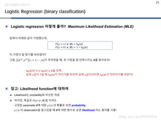
▣ Logistic regression 어떻게 풀까? Maximum Likelihood Estimation (MLE)
앞에서 아래와 같이 가정했는데..
이 가정이 잘 맞기를 바라잖아?
그럼, 𝒙𝒙 𝑖𝑖
, 𝑦𝑦 𝑖𝑖
𝑖𝑖 = 1, ⋯ , 𝑚𝑚}가 주어졌을 때, 위 가정을 잘 만족시키는 𝜽𝜽를 찾아보자!
▣ 참고: Likelihood function에 대하여
▲ Likelihood는 probability와 비슷한 개념
▲ 하지만, 똑같은 𝑃𝑃 𝑦𝑦 𝒙𝒙 ; 𝜽𝜽)일 지라도
고정된 parameter 𝜽𝜽에 대한 𝑦𝑦 | 𝒙𝒙 의 확률로 보면 probability,
𝑦𝑦 | 𝒙𝒙 의 observation을 알고있을 때 𝜽𝜽에 대한 함수로 보면 likelihood 라는 용어를 사용!
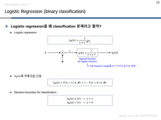
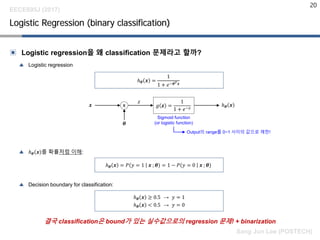
Logistic Regression (binary classification)
𝑃𝑃 𝑦𝑦 = 1 𝒙𝒙 ; 𝜽𝜽) = ℎ𝜽𝜽 𝒙𝒙
𝑃𝑃 𝑦𝑦 = 0 𝒙𝒙 ; 𝜽𝜽) = 1 − ℎ𝜽𝜽 𝒙𝒙
EECE695J (2017)
Sang Jun Lee (POSTECH)
ℎ𝜽𝜽 𝒙𝒙 는 0 ≤ ℎ𝜽𝜽 𝒙𝒙 ≤ 𝟏𝟏을 만족,
실제 𝑦𝑦값이 1일 때 ℎ𝜽𝜽 𝒙𝒙 가 커지기를 바라며 실제 𝑦𝑦값이 0이면 ℎ𝜽𝜽 𝒙𝒙 가 작아지기를 바란다!

21. 22
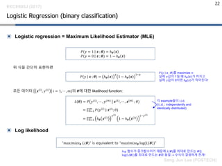
▣ Logistic regression = Maximum Likelihood Estimator (MLE)
위 식을 간단히 표현하면
모든 데이터 𝒙𝒙 𝑖𝑖
, 𝑦𝑦 𝑖𝑖
𝑖𝑖 = 1, ⋯ , 𝑚𝑚}의 𝜽𝜽에 대한 likelihood function:
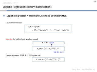
▣ Log likelihood
Logistic Regression (binary classification)
𝑃𝑃 𝑦𝑦 = 1 𝒙𝒙 ; 𝜽𝜽) = ℎ𝜽𝜽 𝒙𝒙
𝑃𝑃 𝑦𝑦 = 0 𝒙𝒙 ; 𝜽𝜽) = 1 − ℎ𝜽𝜽 𝒙𝒙
𝑃𝑃 𝑦𝑦 𝒙𝒙 ; 𝜽𝜽) = ℎ𝜽𝜽 𝒙𝒙
𝑦𝑦
1 − ℎ𝜽𝜽 𝒙𝒙
1−𝑦𝑦
𝐿𝐿 𝜽𝜽 = 𝑃𝑃 𝑦𝑦(1)
, ⋯ , 𝑦𝑦(𝑚𝑚)
𝒙𝒙(1)
, ⋯ , 𝒙𝒙 𝑚𝑚
; 𝜃𝜃)
= ∏𝑖𝑖=1
𝑚𝑚
𝑃𝑃(𝑦𝑦 𝑖𝑖
| 𝒙𝒙(𝑖𝑖)
; 𝜃𝜃)
= ∏𝑖𝑖=1
𝑚𝑚
ℎ𝜽𝜽 𝒙𝒙(𝑖𝑖)
𝑦𝑦(𝑖𝑖)
1 − ℎ𝜽𝜽 𝒙𝒙(𝑖𝑖)
1−𝑦𝑦(𝑖𝑖)
각 example들이 i.i.d.
(i.i.d. : independently and
identically distributed)
“𝑚𝑚𝑚𝑚𝑚𝑚𝑚𝑚 𝑚𝑚𝑚𝑚𝑚𝑚𝑒𝑒𝜽𝜽 𝐿𝐿(𝜽𝜽)” is equivalent to “𝑚𝑚𝑚𝑚𝑚𝑚𝑚𝑚𝑚𝑚𝑚𝑚𝑚𝑚𝑒𝑒𝜽𝜽 log(𝐿𝐿 𝜽𝜽 )”
𝑙𝑙𝑙𝑙𝑙𝑙 함수가 증가함수이기 때문에 𝐿𝐿(𝜽𝜽)를 최대로 만드는 𝜽𝜽는
log(L 𝜽𝜽 )를 최대로 만드는 𝜽𝜽와 동일 → 수식이 깔끔하게 전개!
EECE695J (2017)
Sang Jun Lee (POSTECH)
𝑃𝑃 𝑦𝑦 𝒙𝒙 ; 𝜽𝜽)를 maximize ≡
실제 𝑦𝑦값이 1일 때 ℎ𝜽𝜽 𝒙𝒙 가 커지고
실제 𝑦𝑦값이 0이면 ℎ𝜽𝜽 𝒙𝒙 가 작아진다!

22. 23
▣ Logistic regression = Maximum Likelihood Estimator (MLE)
Log likelihood function:
Maximize the log likelihood: gradient ascent
Logistic regression 문제를 풀기 위한 update rule:
Logistic Regression (binary classification)
𝑙𝑙 𝜽𝜽 = log 𝐿𝐿 𝜽𝜽
= ∑𝑖𝑖=1
𝑚𝑚
𝑦𝑦(𝑖𝑖)
log ℎ𝜽𝜽(𝒙𝒙 𝑖𝑖
) + (1 − 𝑦𝑦 𝑖𝑖
) log(1 − ℎ𝜽𝜽(𝒙𝒙 𝑖𝑖
))
𝜽𝜽 ≔ 𝜽𝜽 + 𝛼𝛼𝛻𝛻𝜽𝜽 𝑙𝑙(𝜽𝜽)
𝛻𝛻𝜽𝜽 𝑙𝑙 𝜽𝜽 = 𝑦𝑦(𝑖𝑖)
− ℎ𝜽𝜽 𝒙𝒙 𝑖𝑖
⋅ 𝒙𝒙 𝑖𝑖
𝜃𝜃𝑗𝑗 ≔ 𝜃𝜃𝑗𝑗 + 𝛼𝛼 𝑦𝑦 𝑖𝑖
− ℎ𝜽𝜽 𝒙𝒙 𝑖𝑖
⋅ 𝑥𝑥𝑗𝑗
𝑖𝑖
직접 계산 해보기!
EECE695J (2017)
Sang Jun Lee (POSTECH)

23. 24
Logistic Regression (binary classification)
𝛻𝛻𝜽𝜽 𝑙𝑙 𝜽𝜽 = 𝑦𝑦(𝑖𝑖)
− ℎ𝜽𝜽 𝒙𝒙 𝑖𝑖
⋅ 𝒙𝒙 𝑖𝑖
Reference: https://www.coursera.org/learn/machine-learning/resources/QQx8l

24. 25
▣ Classification에서 사용되는 cost function을 cross-entropy loss라고 부르는데.. 왜?
Maximize log likelihood function 𝑙𝑙(𝜽𝜽):
is equivalent to
Minimize cross-entropy: 𝑙𝑙𝑙𝑙𝑙𝑙𝑙𝑙 𝜽𝜽 = ∑𝑖𝑖=1
𝑚𝑚
𝐻𝐻 ℎ𝜽𝜽 𝒙𝒙 𝑖𝑖
, 𝑦𝑦 𝑖𝑖
Logistic Regression (binary classification)
𝐻𝐻 ℎ𝜽𝜽 𝒙𝒙 𝑖𝑖
, 𝑦𝑦 𝑖𝑖
= −𝑦𝑦 𝑖𝑖
log ℎ𝜽𝜽 𝒙𝒙 𝑖𝑖
− (1 − 𝑦𝑦 𝑖𝑖
) log(1 − ℎ𝜽𝜽(𝒙𝒙 𝑖𝑖
))
Cross-entropy loss :
𝑙𝑙 𝜽𝜽 = ∑𝑖𝑖=1
𝑚𝑚
𝑦𝑦(𝑖𝑖)
log ℎ𝜽𝜽(𝒙𝒙 𝑖𝑖
) + (1 − 𝑦𝑦 𝑖𝑖
) log(1 − ℎ𝜽𝜽(𝒙𝒙 𝑖𝑖
))
Log likelihood function :
𝑦𝑦(𝑖𝑖) = 1이면 − log ℎ𝜽𝜽(𝒙𝒙 𝑖𝑖 )의 loss를
𝑦𝑦(𝑖𝑖) = 0이면 −log(1 − ℎ𝜽𝜽(𝒙𝒙 𝑖𝑖 ))의 loss를 부여
EECE695J (2017)
Sang Jun Lee (POSTECH)

25. 26
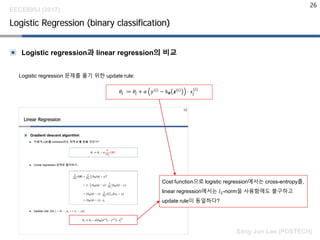
▣ Logistic regression과 linear regression의 비교
Logistic regression 문제를 풀기 위한 update rule:
Logistic Regression (binary classification)
𝜃𝜃𝑗𝑗 ≔ 𝜃𝜃𝑗𝑗 + 𝛼𝛼 𝑦𝑦 𝑖𝑖
− ℎ𝜽𝜽 𝒙𝒙 𝑖𝑖
⋅ 𝑥𝑥𝑗𝑗
𝑖𝑖
EECE695J (2017)
Sang Jun Lee (POSTECH)
Cost function으로 logistic regression에서는 cross-entropy를,
linear regression에서는 𝑙𝑙2-norm을 사용함에도 불구하고
update rule이 동일하다?

26. 27
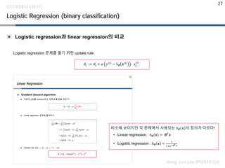
▣ Logistic regression과 linear regression의 비교
Logistic regression 문제를 풀기 위한 update rule:
Logistic Regression (binary classification)
𝜃𝜃𝑗𝑗 ≔ 𝜃𝜃𝑗𝑗 + 𝛼𝛼 𝑦𝑦 𝑖𝑖
− ℎ𝜽𝜽 𝒙𝒙 𝑖𝑖
⋅ 𝑥𝑥𝑗𝑗
𝑖𝑖
비슷해 보이지만 각 문제에서 사용되는 ℎ𝜽𝜽 𝒙𝒙 의 정의가 다르다!
• Linear regression : ℎ𝜽𝜽 𝒙𝒙 = 𝜽𝜽𝑇𝑇
𝒙𝒙
• Logistic regression : ℎ𝜽𝜽 𝒙𝒙 =
1
1+𝑒𝑒−𝜽𝜽 𝑇𝑇 𝒙𝒙
EECE695J (2017)
Sang Jun Lee (POSTECH)

27. 28
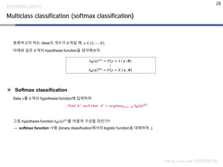
분류하고자 하는 class의 개수가 𝐾𝐾개일 때: 𝑦𝑦 ∈ {1, ⋯ , 𝐾𝐾}
아래와 같은 𝐾𝐾개의 hypothesis function을 생각해보자
▣ Softmax classification
Data 𝑥𝑥를 𝐾𝐾개의 hypothesis function에 입력하여
𝐹𝐹𝑖𝑖𝑖𝑖𝑖𝑖 𝑘𝑘∗
𝑠𝑠𝑠𝑠𝑠𝑠𝑠 𝑡𝑡 𝑡𝑡𝑡𝑡𝑡 𝑘𝑘∗
= 𝑎𝑎𝑎𝑎𝑎𝑎𝑎𝑎𝑎𝑎𝑥𝑥𝑘𝑘=1,⋯,𝐾𝐾 ℎ𝜽𝜽 𝒙𝒙 (𝑘𝑘)
그럼 hypothesis function ℎ𝜽𝜽 𝒙𝒙 (𝑘𝑘)
를 어떻게 구성할 것인가?
→ softmax function 사용 (binary classification에서의 logistic function을 대체하여..)
Multiclass classification (softmax classification)
ℎ𝜽𝜽 𝒙𝒙 (1)
= 𝑃𝑃 𝑦𝑦 = 1 𝒙𝒙 ; 𝜽𝜽)
⋮
ℎ𝜽𝜽 𝒙𝒙 (𝐾𝐾)
= 𝑃𝑃 𝑦𝑦 = 𝐾𝐾 𝒙𝒙 ; 𝜽𝜽)
EECE695J (2017)
Sang Jun Lee (POSTECH)

28. 29
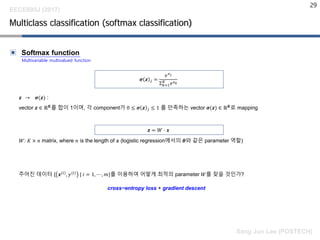
▣ Softmax function
𝒛𝒛 → 𝝈𝝈(𝒛𝒛) :
vector 𝒛𝒛 ∈ ℝ𝑲𝑲
를 합이 1이며, 각 component가 0 ≤ 𝝈𝝈 𝒛𝒛 𝑗𝑗 ≤ 1 를 만족하는 vector 𝝈𝝈(𝒛𝒛) ∈ ℝ𝑲𝑲
로 mapping
𝑊𝑊: 𝐾𝐾 × 𝑛𝑛 matrix, where 𝑛𝑛 is the length of 𝒙𝒙 (logistic regression에서의 𝜽𝜽와 같은 parameter 역할)
주어진 데이터 { 𝒙𝒙(𝑖𝑖)
, 𝑦𝑦(𝑖𝑖)
| 𝑖𝑖 = 1, ⋯ , 𝑚𝑚}를 이용하여 어떻게 최적의 parameter 𝑊𝑊를 찾을 것인가?
Multiclass classification (softmax classification)
𝝈𝝈 𝒛𝒛 𝑗𝑗 =
𝑒𝑒 𝑧𝑧𝑗𝑗
Σ𝑘𝑘=1
𝐾𝐾
𝑒𝑒 𝑧𝑧𝑘𝑘
Multivariable multivalued function
𝒛𝒛 = 𝑊𝑊 ⋅ 𝒙𝒙
cross−entropy loss + gradient descent
EECE695J (2017)
Sang Jun Lee (POSTECH)

29. 30
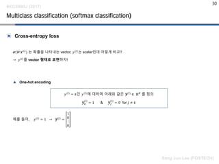
▣ Cross-entropy loss
𝝈𝝈(𝑊𝑊𝒙𝒙(𝑖𝑖)
) 는 확률을 나타내는 vector, 𝑦𝑦(𝑖𝑖)
는 scalar인데 어떻게 비교?
→ 𝑦𝑦(𝑖𝑖)
를 vector 형태로 표현하자!
▲ One-hot encoding
예를 들어, 𝑦𝑦(𝑖𝑖)
= 1 → �𝒚𝒚(𝑖𝑖)
=
1
0
⋮
0
Multiclass classification (softmax classification)
𝑦𝑦(𝑖𝑖)
= 𝑘𝑘인 𝑦𝑦(𝑖𝑖)
에 대하여 아래와 같은 �𝒚𝒚(𝑖𝑖)
∈ ℝ𝐾𝐾
를 정의
�𝒚𝒚𝑘𝑘
(𝑖𝑖)
= 1 & �𝒚𝒚𝑗𝑗
(𝑖𝑖)
= 0 for 𝑗𝑗 ≠ 𝑘𝑘
EECE695J (2017)
Sang Jun Lee (POSTECH)

30. 31
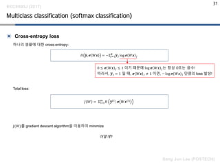
▣ Cross-entropy loss
하나의 샘플에 대한 cross-entropy:
Total loss:
𝐽𝐽(𝑊𝑊)를 gradient descent algorithm을 이용하여 minimize
Multiclass classification (softmax classification)
𝐻𝐻 �𝒚𝒚, 𝝈𝝈 𝑊𝑊𝒙𝒙 = −Σ𝑗𝑗=1
𝐾𝐾
�𝒚𝒚𝑗𝑗 log 𝝈𝝈 𝑊𝑊𝒙𝒙 𝑗𝑗
0 ≤ 𝝈𝝈 𝑊𝑊𝒙𝒙 𝑗𝑗 ≤ 1 이기 때문에 log 𝝈𝝈 𝑊𝑊𝒙𝒙 𝑗𝑗는 항상 0또는 음수!
따라서, �𝒚𝒚𝑗𝑗 = 1 일 때, 𝝈𝝈 𝑊𝑊𝒙𝒙 𝑗𝑗 ≠ 1 이면, − log 𝝈𝝈 𝑊𝑊𝒙𝒙 𝑗𝑗 만큼의 loss 발생!
𝐽𝐽 𝑊𝑊 = Σ𝑖𝑖=1
𝑚𝑚
𝐻𝐻 �𝒚𝒚(𝑖𝑖)
, 𝝈𝝈 𝑊𝑊𝒙𝒙(𝑖𝑖)
어떻게?
EECE695J (2017)
Sang Jun Lee (POSTECH)

31. 32
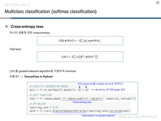
▣ Cross-entropy loss
하나의 샘플에 대한 cross-entropy:
Total loss:
𝐽𝐽(𝑊𝑊)를 gradient descent algorithm을 이용하여 minimize
어떻게? → TensorFlow in Python!
Multiclass classification (softmax classification)
𝐻𝐻 �𝒚𝒚, 𝝈𝝈 𝑊𝑊𝒙𝒙 = −Σ𝑗𝑗=1
𝐾𝐾
�𝒚𝒚𝑗𝑗 log 𝝈𝝈 𝑊𝑊𝒙𝒙 𝑗𝑗
𝐽𝐽 𝑊𝑊 = Σ𝑖𝑖=1
𝑚𝑚
𝐻𝐻 �𝒚𝒚(𝑖𝑖)
, 𝝈𝝈 𝑊𝑊𝒙𝒙(𝑖𝑖)
EECE695J (2017)
Sang Jun Lee (POSTECH)
먼저 parameter를 variable tensor로 정의하고
𝝈𝝈 𝑊𝑊𝒙𝒙 𝑗𝑗에 대한 graph 생성
Cross-entropy loss
Optimization via gradient descent

32. 33
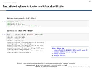
TensorFlow implementation for multiclass classification
MNIST dataset load
• trainimg: 55000x784 (28x28 영상을 784 length의 vector로..)
• trainlabel: 55000x10 (one-hot encoding)
• testimg: 10000x784
• testlabel: 10000x10
Code is available at: 141.223.87.129data상준EECE695J_딥러닝기초및활용
File name: W2_softmax_classification.ipynb
Reference: https://github.com/sjchoi86/tensorflow-101/blob/master/notebooks/logistic_regression_mnist.ipynb
EECE695J (2017)
Sang Jun Lee (POSTECH)

33. 34
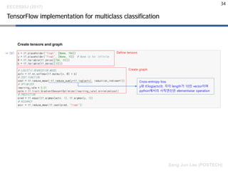
TensorFlow implementation for multiclass classification
Cross-entropy loss
y와 tf.log(actv)는 각각 length가 10인 vector이며
python에서의 사칙연산은 elementwise operation
Define tensors
Create graph
EECE695J (2017)
Sang Jun Lee (POSTECH)

34. 35
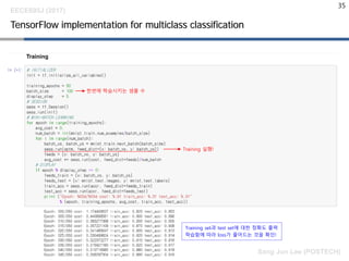
TensorFlow implementation for multiclass classification
한번에 학습시키는 샘플 수
Training 실행!
Training set과 test set에 대한 정확도 출력
학습함에 따라 loss가 줄어드는 것을 확인!
EECE695J (2017)
Sang Jun Lee (POSTECH)

35. 36
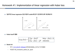
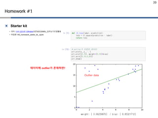
▲ 일반적인 linear regression 알고리즘이 outlier에 좀 더 강인해지도록 개선해보자!
▲ Huber loss의 활용
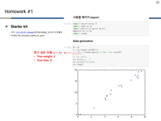
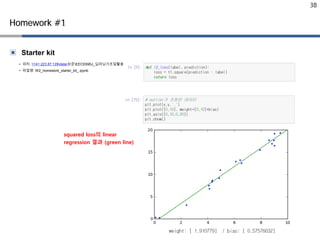
▲ Starter kit
• 위치: 141.223.87.129data상준EECE695J_딥러닝기초및활용
• 파일명: W2_homework_starter_kit_.ipynb
Homework #1: Implementation of linear regression with Huber loss

36. 37
▣ Starter kit
Homework #1
찾고 싶은 모델: 𝒚𝒚 = 𝟐𝟐𝟐𝟐
• True weight: 2
• True bias: 0
• 위치: 141.223.87.129data상준EECE695J_딥러닝기초및활용
• 파일명: W2_homework_starter_kit_.ipynb

37. 38
▣ Starter kit
Homework #1
squared loss의 linear
regression 결과 (green line)
• 위치: 141.223.87.129data상준EECE695J_딥러닝기초및활용
• 파일명: W2_homework_starter_kit_.ipynb

38. 39
▣ Starter kit
Homework #1
데이터에 outlier가 존재하면?
Outlier data
• 위치: 141.223.87.129data상준EECE695J_딥러닝기초및활용
• 파일명: W2_homework_starter_kit_.ipynb

39. 40
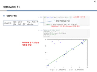
▣ Starter kit
Homework #1
Homework!
delta값은 1을 사용
Huber loss 구현에 있어서 tf.select 함수를 참조
Outlier에 좀 더 강인한
특성을 보임!

40. 41
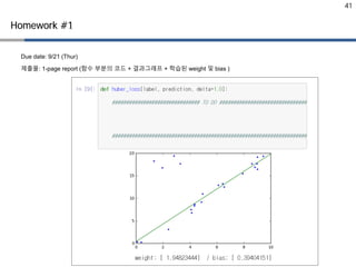
Due date: 9/21 (Thur)
제출물: 1-page report (함수 부분의 코드 + 결과그래프 + 학습된 weight 및 bias )
Homework #1

41. 42
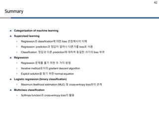
▲ Categorization of machine learning
▲ Supervised learning
• Regression과 classification에 대한 loss 관점에서의 이해
• Regression: prediction과 정답이 얼마나 다른가를 loss로 사용
• Classification: 정답과 다른 prediction에 대하여 동일한 크기의 loss 부여
▲ Regression
• Regression 문제를 풀기 위한 두 가지 방법
• Iterative method로서의 gradient descent algorithm
• Explicit solution을 찾기 위한 normal equation
▲ Logistic regression (binary classification)
• Maximum likelihood estimation (MLE) 및 cross-entropy loss와의 관계
▲ Multiclass classification
• Softmax function과 cross-entropy loss의 활용
Summary

42. 43
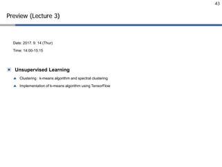
Date: 2017. 9. 14 (Thur)
Time: 14:00-15:15
▣ Unsupervised Learning
▲ Clustering : k-means algorithm and spectral clustering
▲ Implementation of k-means algorithm using TensorFlow
Preview (Lecture 3)