Denoising auto encoder와 Stacked auto encoder관련 발표 자료

1. Denoising Auto encoders(dA)
Produce by Tae Young Lee

2. history
• 1958 Rosenblatt proposed perceptrons
• 1980 Neocognitron (Fukushima, 1980)
• 1982 Hopfield network, SOM (Kohonen, 1982),
Neural PCA (Oja, 1982)
• 1985 Boltzmann machines (Ackley et al., 1985)
• 1986 Multilayer perceptrons and backpropagation
(Rumelhart et al., 1986)
1988 RBF networks (Broomhead&Lowe, 1988)
• 1989 Autoencoders (Baldi&Hornik, 1989),
Convolutional network (LeCun, 1989)
1992 Sigmoid belief network (Neal, 1992)
• 1993 Sparse coding (Field, 1993)

3. Beyond the Wall
deep learning beyond the limits

4. Limitation
• First.
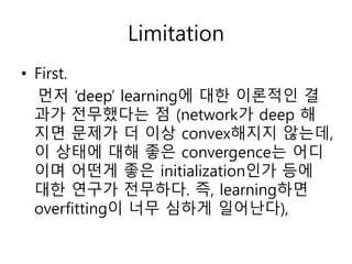
먼저 ‘deep’ learning에 대한 이론적인 결
과가 전무했다는 점 (network가 deep 해
지면 문제가 더 이상 convex해지지 않는데,
이 상태에 대해 좋은 convergence는 어디
이며 어떤게 좋은 initialization인가 등에
대한 연구가 전무하다. 즉, learning하면
overfitting이 너무 심하게 일어난다),

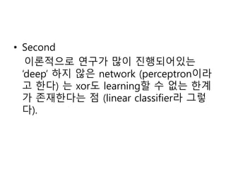
5. • Second
이론적으로 연구가 많이 진행되어있는
‘deep’ 하지 않은 network (perceptron이라
고 한다) 는 xor도 learning할 수 없는 한계
가 존재한다는 점 (linear classifier라 그렇
다).

6. Overcome
• 가장 크게 차이 나는 점은 예전과는 다르
게 overfitting을 handle할 수 있는 좋은 연
구가 많이 나오게 되었다. 처음 2007, 2008
년에 등장했던 unsupervised pre-training
method들 (이 글에서 다룰 내용들), 2010
년도쯤 들어서서 나오기 시작한 수많은
regularization method들 (dropout, ReLU
등).

7. • Third
computation cost가 무시무시해서 그 당
시 컴퓨터로는 도저히 처리할 엄두조차 낼
수 없었다는 점이다.
Limitation

8. Overcome
• 하드웨어 스펙이 압도적으로 뛰어난데다가, GPU
parallelization에 대한 이해도가 높아지게 되면서
에전과는 비교도 할 수 없을 정도로 많은
computation power를 사용할 수 있게 되었다
• 현재까지 알려진 바로는 network가 deep할 수록
그 최종적인 성능이 좋아지며, optimization을 많
이 하면 할 수록 그 성능이 좋아지기 때문에,
computation power를 더 많이 사용할 수 있다면
그만큼 더 좋은 learning을 할 수 있다는 것을 의
미한다.

9. Denoising Auto Encoder
Image Processing

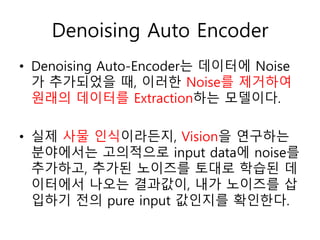
13. Denoising Auto Encoder
• Denoising Auto-Encoder는 데이터에 Noise
가 추가되었을 때, 이러한 Noise를 제거하여
원래의 데이터를 Extraction하는 모델이다.
• 실제 사물 인식이라든지, Vision을 연구하는
분야에서는 고의적으로 input data에 noise를
추가하고, 추가된 노이즈를 토대로 학습된 데
이터에서 나오는 결과값이, 내가 노이즈를 삽
입하기 전의 pure input 값인지를 확인한다.

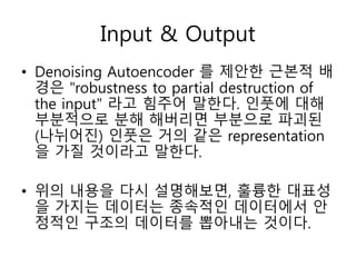
14. Input & Output
• Denoising Autoencoder 를 제안한 근본적 배
경은 "robustness to partial destruction of
the input" 라고 힘주어 말한다. 인풋에 대해
부분적으로 분해 해버리면 부분으로 파괴된
(나뉘어진) 인풋은 거의 같은 representation
을 가질 것이라고 말한다.
• 위의 내용을 다시 설명해보면, 훌륭한 대표성
을 가지는 데이터는 종속적인 데이터에서 안
정적인 구조의 데이터를 뽑아내는 것이다.

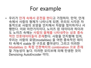
15. For example
• 우리가 안개 속에서 운전을 한다고 가정하자. 만약, 안개
속에서 사람의 형체가 나타나게 되면, 우리의 시각은 자
동적으로 사람의 모양을 인지해서 차량을 정지하거나 서
행한다. 이와 마찬가지이다, 노이즈 된 데이터라 하더라
도 노이즈 속에는 사람의 물체를 나타내주는 상호 종속
적인 인풋데이터들이 존재한다. 사람을 인지함에 있어,
우리는 사람의 모양(modalities) 을 어떤 종속적인 데이
터 속에서 stable 한 구조로 뽑아낸다. 그리고 이러한
Modalities 는 특정 인풋벡터의 combination 으로 존재
할 가능성이 높다. 이러한 모티브에 의해 탄생한 것이
Denoising AutoEncoder 이다.

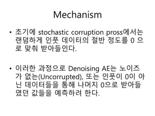
16. Mechanism
• 초기에 stochastic corruption pross에서는
랜덤하게 인풋 데이터의 절반 정도를 0 으
로 맞춰 받아들인다.
• 이러한 과정으로 Denoising AE는 노이즈
가 없는(Uncorrupted), 또는 인풋이 0이 아
닌 데이터들을 통해 나머지 0으로 받아들
였던 값들을 예측하려 한다.

17. Stacked Denoising
Autoencoders

18. Stacked Autoencoder(1)
• Stacked Autoencoder가 Autoencoder에 비해 갖는 가장
큰 차이점은 DBN(Deep Belief Network)의 구조라는 것
이다.
• 기존의 AE는 BP(BackPropagation)를 활용하여 Weight를
학습하였다. 하지만 이는 Layer와 Unit의 개수가 많아지
면 많아질 수록 Weight를 학습하는데 방대한 계산량과
Local Minima 에 빠질 위험이 존재한다. 또한 지속적으
로 작은 값들이 Update 되는 과정에서 Weight의 오차가
점점 줄어드는 이른바, Vanishing Gradient의 문제를 갖
고 있다.

19. • * DBN(Deep Belief Network)에서는 RBM(Restricted Boltzmann Machine)을 도입한
다.
RBM은 Fully connected Boltzmann Machine을 변형한 것으로, Unit의 Inner
Connection을 제한한 모델로, Layer과 Layer 사이의 Connection 만 존재하는 모델이
다. RBM에서는 BP 방법이 아니라, (Alternative) Gibbs sampling을 활용한
Contrastive Divergence(CD) 를 활용하여 Maximum Likelihood Estimation (MLE) 문
제를 해결하였다. CD트레이닝 방법은 위에서 언급한 MLE 뿐만 아니라, 트레이닝 샘
플의 확률 분포 함수와 모델의 확률 분포 함수의 Kullback-Leibler Divergence를 이용
한 식의 Gradient-Descent 방법을 통해 유도 할 수 있다.
• 핵심적인 idea 는 모델링을 함에 있어서 p(y=label|x=data)p(y=label|x=data) 가 아니
라, p(data)p(data) 만을 가지고도 layer 가 label 을 generate 할 수 있도록
Generative Model 을 만드는 것이다. 이 말은 곧, Training Data에서 Input과 Output
이 필요하지 않기 때문에, Unsupervised Learning과 Semi-Supervised Learning에 적
용할 수 있게 되었다.
• 이러한 DBN모델에서 층별로 학습시키는 방법을 [Bengio]가 본인의 논문 "Greedy
Layer-Wise Training of Deep Networks(2007)"에서 제안한다. 그리고 이를 활용한 모
델이 바로 Stacked AE 이다. 그리고 이러한 학습 방식을 Greedy Layer-Wise Training
라고 한다.
Stacked Autoencoder(2)

20. Stacked Autoencoder 장/단점
• Stacked Auto-Encoders(SAE)에서는 완전하게 Deep Generative
Model 이라고 할 수 없는 것이, RBM에서는 probabilistic 에 의존하
여, data만 가지고도 label 을 관측하려 하는데, SAE에서는 사실상
deterministic 방법으로 모델을 학습한다.
p(h=0,1)=s(Wx+b)p(h=0,1)=s(Wx+b) 가 아니라,
h=s(Wx+b)h=s(Wx+b) 로 학습한다.
• 이에 따른 단점으로는 완벽한 Deep Generative Model 은 아니라는
것이지만,
• 장점은 training 에 속도가 빠르고, Deep Neural Nets 의 속성들을
이용할 수 있다는 것이다.

21. Vanishing gradient 문제
• Vanishing gradient 문제는 1991년에 Sepp Hochreiter에 의해 발견
• Vanishing gradient 문제가 더 많은 관심을 받은 이유는 두 가지인데,
하나는 exploding gradient 문제는 쉽게 알아차릴 수 있다는 점이다.
Gradient 값들이 NaN (not a number)이 될 것이고 프로그램이 죽을
것이기 때문이다. 두 번째는, gradient 값이 너무 크다면 미리 정해
준 적당한 값으로 잘라버리는 방법 (이 논문에서 다뤄졌다)이 매우
쉽고 효율적으로 이 문제를 해결하기 때문이다. Vanishing gradient
문제는 언제 발생하는지 바로 확인하기가 힘들고 간단한 해결법이
없기 때문에 더 큰 문제였다.

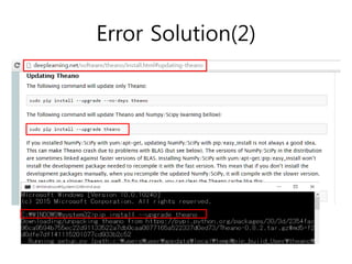
22. Vanishing gradient 문제 해결
• W 행렬을 적당히 좋은 값으로 잘 초기화 해준다면 vanishing
gradient의 영향을 줄일 수 있고, regularization을 잘 정해줘도 비슷
한 효과를 볼 수 있다. 더 보편적으로 사용되는 방법은 tanh나
sigmoid activation 함수 말고 ReLU를 사용하는 것이다. ReLU는 미
분값의 최대치가 1로 정해져있지 않기 때문에 gradient 값이 없어져
버리는 일이 크게 줄어든다. 이보다 더 인기있는 해결책은 Long
Short-Term Memory (LSTM)이나 Gated Recurrent Unit (GRU) 구조
를 사용하는 방법이다. LSTM은 1997년에 처음 제안되었고, 현재 자
연어처리 분야에서 가장 널리 사용되는 모델 중 하나이다. GRU
는 2014년에 처음 나왔고, LSTM을 간략화한 버전이다. 두 RNN의
변형 구조 모두 vanishing gradient 문제 해결을 위해 디자인되었고,
효과적으로 긴 시퀀스를 처리할 수 있다는 것이 보여졌다.

23. Auto Encoder R Source

24. (theano) 8 Stacked Denoising
Autoencoders (SdA)

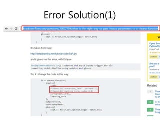
28. Error occurred
C:DevelopEnvironmentPython27python.exe "C:/DevelopEnvironment/PyCharm
Community Edition 4.0.4/Source_Repository/DeepLearningTutorials-
master/code/SdA.py"
... loading data
... building the model
... getting the pretraining
functions Traceback (most recent call last): File "C:/DevelopEnvironment/PyCharm
Community Edition 4.0.4/Source_Repository/DeepLearningTutorials-
master/code/SdA.py", line 491, in <module> test_SdA() File
"C:/DevelopEnvironment/PyCharm Community Edition
4.0.4/Source_Repository/DeepLearningTutorials-master/code/SdA.py", line 382, in
test_SdA batch_size=batch_size) File "C:/DevelopEnvironment/PyCharm Community
Edition 4.0.4/Source_Repository/DeepLearningTutorials-master/code/SdA.py", line
226, in pretraining_functions self.x: train_set_x[batch_begin: batch_end] File
"C:DevelopEnvironmentPython27libsite-
packagestheanocompilefunction.py", line 248, in function "In() instances
and tuple inputs trigger the old " NotImplementedError: In() instances and
tuple inputs trigger the old semantics, which disallow using updates and
givens

30. Error Solution(1)

31. Error Solution(2)

32. Success

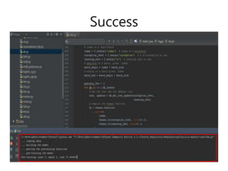
33. if __name__ == '__main__':
test_SdA()
def test_SdA(finetune_lr=0.1, pretraining_epochs=15,
pretrain_lr=0.001, training_epochs=1000,
dataset='mnist.pkl.gz', batch_size=1):
datasets = load_data(dataset)
train_set_x, train_set_y = datasets[0]
valid_set_x, valid_set_y = datasets[1]
test_set_x, test_set_y = datasets[2]
# construct the stacked denoising autoencoder class
sda = SdA(
numpy_rng=numpy_rng,
n_ins=28 * 28,
hidden_layers_sizes=[1000, 1000, 1000],
n_outs=10
)
pretraining_fns = sda.pretraining_functions(train_set_x=train_set_x,
batch_size=batch_size)
## Pre-train layer-wise
corruption_levels = [.1, .2, .3]
for i in range(sda.n_layers):
# go through pretraining epochs
for epoch in range(pretraining_epochs):
# go through the training set
c = []
for batch_index in range(n_train_batches):
c.append(pretraining_fns[i](index=batch_index,
corruption=corruption_levels[i],
lr=pretrain_lr))
print('Pre-training layer %i, epoch %d, cost %f' % (i, epoch, numpy.mean(c)))
end_time = timeit.default_timer()

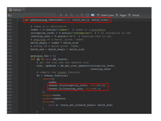
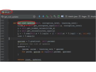
34. def pretraining_functions(self, train_set_x, batch_size):
# index to a [mini]batch
index = T.lscalar('index') # index to a minibatch
corruption_level = T.scalar('corruption') # % of corruption to use
learning_rate = T.scalar('lr') # learning rate to use
# begining of a batch, given `index`
batch_begin = index * batch_size
# ending of a batch given `index`
batch_end = batch_begin + batch_size
pretrain_fns = []
for dA in self.dA_layers:
# get the cost and the updates list
cost, updates = dA.get_cost_updates(corruption_level,
learning_rate)
# compile the theano function
fn = theano.function(
inputs=[
index,
theano.In(corruption_level, value=0.2),
theano.In(learning_rate, value=0.1)
],
outputs=cost,
updates=updates,
givens={
self.x: train_set_x[batch_begin: batch_end]
}
)
# append `fn` to the list of functions
pretrain_fns.append(fn)
return pretrain_fns