Aryal.pdf

Mobile Hyperspectral Imaging for
Material Surface Damage Detection
Sameer Aryal1
; ZhiQiang Chen, M.ASCE2
; and Shimin Tang3
Abstract: Many machine vision–based inspection methods aim to replace human-based inspection with an automated or highly efficient
procedure. However, these machine-vision systems have not been endorsed entirely by civil engineers for deployment in practice, partially
due to their poor performance in detecting damage amid other complex objects on material surfaces. This work developed a mobile hyper-
spectral imaging system which captures hundreds of spectral reflectance values in a pixel in the visible and near-infrared (VNIR) portion of
the electromagnetic spectrum. To prove its potential in discriminating complex objects, a machine learning methodology was developed with
classification models that are characterized by four different feature extraction processes. Experimental validation showed that hyperspectral
pixels, when used conjunctly with dimensionality reduction, possess outstanding potential for recognizing eight different surface objects
(e.g., with an F1 score of 0.962 for crack detection), and outperform gray-valued images with a much higher spatial resolution. The authors
envision the advent of computational hyperspectral imaging for automating damage inspection for structural materials, especially when
dealing with complex scenes found in built objects in service. DOI: 10.1061/(ASCE)CP.1943-5487.0000934. © 2020 American Society
of Civil Engineers.
Author keywords: Machine vision; Hyperspectral imaging; Damage detection; Machine learning; Dimensionality reduction.
Introduction
Civil engineering structures are vital for a society’s prosperity and
quality of life in general. To ensure the serviceability and safety of
structures, different technology-based inspection and monitoring
methods have been researched. These technologies generally can
be categorized into two types. The first is nondestructive evaluation
(NDE) through advanced sensing technologies (e.g., X-ray, micro-
wave, thermal, and ultrasonic imaging) (Cawley 2018), most of
which aim to detect subsurface anomalies or damage. The second
category includes various structural health monitoring (SHM)
methods (Sohn et al. 2003), which seek to monitor the dynamic
responses and identify the intrinsic parameters or changes in struc-
tures. Even with these technology-based inspection or monitoring
methods, the reality is that, at least for transportation structures that
are managed by DOT agencies in most states in the US, manual or
visual inspection is considered the mainstream approach (Olsen
et al. 2016). This mainly is because surface damage (e.g., cracks
and corrosion) on structural materials, compared with subsurface
damage, is more commonplace and can be viewed as a clue to in-
ternal damage or possible degrading of the system integrity. For
bridges, standard manuals and guidelines exist for practical
inspection, including the Manual for Bridge Element Inspection
(AASHTO 2019) and the Guidelines for Inspecting Complex Com-
ponents of Bridges (Leshko 2002). Due to the low cost and ubiqui-
tous availability of optical sensors (i.e., digital cameras), it is no
surprise that optical imaging has become widely adopted for struc-
tural inspection, wherein digital images are recorded for records or
postinspection analysis (Olsen et al. 2016). Subsequently, this has
motivated the development of machine vision techniques to aid or
automate engineering inspection for civil structures.
Machine vision is a technical field that concerns the develop-
ment of digital imaging methods and the use of image processing
or computer vision algorithms for the extraction of useful informa-
tion from images (Morris 2004). With the advent of early digital
cameras, researchers in the 1980s and 1990s used simple digital
filters, including various edge-detection methods, for image-based
damage detection for structural materials (Cheng and Miyojim
1998; Ritchie 1987; Ritchie 1990). To further automate the process
of image capturing, researchers also strive to develop operationally
efficient methods that are expected to mitigate the human cost.
These methods include ground vehicle–based imaging, aerial ve-
hicle–based imaging, and crowdsourcing-based imaging (e.
g., Isawa et al. 2005; Kim et al. 2015; Lattanzi and Miller
2013; Ozer et al. 2015; Tung et al. 2002; Zhang and Elaksher
2012). For example, Ho et al. (2013) developed a system with
three cameras attached to a cable-climbing robot to detect surface
damage. Yeum and Dyke (2015) proposed the use of unmanned
aerial vehicles (UAVs) for remote imaging and damage detection.
Chen et al. (2015) proposed a mobile-cloud infrastructure enabled
approach that exploits collaborative mobile and cloud computing to
harness crowdsourcing for damage inspection.
With the abundance of these optical imaging platforms, one prom-
ising fact is the ease of obtaining imagery databases. Besides the ba-
sic image processing methods, these databases enable the adoption of
a machine learning (ML) paradigm. To this end, many machine learn-
ing methods feature the use of supervised or nonsupervised classi-
fiers (Chen et al. 2011; Gavilán et al. 2011; Kaseko and Ritchie
1993; Liu et al. 2002; Prasanna et al. 2014; Zakeri et al. 2017).
1
Graduate Student, Dept. of Civil and Mechanical Engineering, Univ. of
Missouri Kansas City, FH 5110 Rockhill Rd., Kansas City, MO 64110.
Email: sayd8@mail.umkc.edu
2
Associate Professor, School of Computing and Engineering, Univ. of
Missouri Kansas City, FH 5110 Rockhill Rd., Kansas City, MO 64110 (cor-
responding author). ORCID: https://orcid.org/0000-0002-0793-0089.
Email: chenzhiq@umkc.edu
3
Ph.D. Candidate, Dept. of Computer Science and Electrical Engineer-
ing, Univ. of Missouri Kansas City, FH 5110 Rockhill Rd., Kansas City,
MO 64110. Email: st78d@mail.umkc.edu
Note. This manuscript was submitted on March 30, 2020; approved on
July 15, 2020; published online on November 9, 2020. Discussion period
open until April 9, 2021; separate discussions must be submitted for indi-
vidual papers. This paper is part of the Journal of Computing in Civil En-
gineering, © ASCE, ISSN 0887-3801.
© ASCE 04020057-1 J. Comput. Civ. Eng.
J. Comput. Civ. Eng., 2021, 35(1): 04020057
Downloaded
from
ascelibrary.org
by
University
of
Liverpool
on
11/14/20.
Copyright
ASCE.
For
personal
use
only;
all
rights
reserved.

In recent years, coincident with the advances in artificial intelli-
gence (AI) and particularly the development of deep learning
(DL) techniques, many have heralded the era of AI-enabled damage
inspection. A simple search through Google Scholar, using the
combined keywords of crack detection, convolutional neural net-
work (CNN), and image returned more than 1,200 articles from
the period January 2016 to May 2020. Zhang et al. (2016) first used
a CNN model as a feature extractor, then fed the features into a
classification model for the detection of cracks in images. Such
a CNN-based machine learning approach then was adopted in
many other similar efforts (e.g., Alipour et al. 2019; Cha et al. 2017;
Ni et al. 2019).
One may expect that by duly considering these advances in
AI-enabled image-based damage detection and the lowering cost
of mobile or edge computing devices, autonomous damage inspec-
tion may become a reality. However, these machine-vision systems
have not been endorsed entirely by civil engineers for deploying
these techniques in practice. The authors argue that if the scene
complexity captured in digital images is not acknowledged, the
pace of automation ultimately would be hindered. In the case of
concrete structures in service, the scenes in images often are a mix-
ture of characteristic material texture, possible damage, and other
artifacts, such as artificial marking, vegetation, moisture, oil spill,
discoloring, and uneven illumination (Chen and Hutchinson 2010).
This implies that any image-based machine learning method or
end-to-end deep learning method may encounter the infamous
issue of generalization. In other words, if such an autonomous
image-based system is deployed in the field, its core detection
component (i.e., a classification model), even one trained based
on a relatively large data set with complex scenes, can overfit
the training data but cannot generalize to the multitude of different
and arbitrary scenes that are not in the prepared data sets for model
training.
To resolve this challenge, one obvious solution is to continue
developing much larger data sets, given the power of deep learning
with an architecture that potentially can accommodate any scale
of data sizes and any complexity in field scenes. However, this
inevitably triggers the issue of labeling big data (e.g., pixelwise
labeling of cracks and other artifacts), which is expensive and
time-consuming (Roh et al. 2019). Another approach is to resort
to transfer learning and use small data sets enhanced by effective
data augmentation techniques to obtain the notion of learning from
small data using DL models. Tang and Chen (2017) developed a
novel data augmentation technique for accommodating deep trans-
fer learning from small data. Regardless of the potential success of
these solutions, with the use of red, green, and blue (RGB) images,
these methods can only asymptotically match the intelligence of
trained inspectors (who provide labeled training data), although
possibly with much higher efficiency than human inspectors. In
other words, there is a performance ceiling that limits the capacity
of regular RGB images unless the machine intelligence supersedes
that of human beings.
An alternative solution is to break out the normal matching of
human vision. An emerging technology for nondestructive inspec-
tion is hyperspectral imaging (HSI). In a hyperspectral image,
a pixel contains tens to thousands of digital values in different
spectral bands in the visible and near-infrared (VNIR) portion of
the electromagnetic spectrum, at which each digital value represents
either the reflectance property or the transmittance property of a
material in one band. Such a high-dimensional spectral profile is
not directly visible to human eyes, which, roughly speaking, re-
spond to three discrete bands (RGB) (Kaiser and Boynton 1996).
Scientific knowledge of hyperspectral imaging and analysis is well
archived in the knowledge body of hyperspectral spectroscopy
(Siesler et al. 2008). In the context of image-based damage detec-
tion, HSI provides a significant possibility of detecting and iden-
tifying the presence of material damage amid complex scenes on
surfaces of civil structures.
The authors developed a mobile hyperspectral imaging system
for both ground and aerial vehicle–based remote sensing. With this
mobile HSI system and preliminary observation (e.g., by plotting
spectral profiles for different material surface objects), it is hypoth-
esized that material damage (e.g., cracks) and other complex arti-
facts on structural surfaces can be detected effectively with high
performance. The ensuing research problem is whether the resulting
machine-learning model based on hyperspectral pixels can outper-
form the same model trained based on regular images with a high
spatial resolution (i.e., those based on panchromatic or true-color
imaging). The essential contribution of this study is the proven ef-
fectiveness of HSI for material damage detection with complex
scenes, and its superb capacity compared with high-resolution pan-
chromatic (gray) images. Specifically, unlike any existing image-
based damage detection method, the proposed machine-learning
framework deals with the detection problem with many semanti-
cally rich structural-surface materials and objects, including con-
crete, asphalt, crack, dry vegetation, green vegetation, water, oil, and
artificial markings. Such a plentiful amount of surface object cat-
egories are not dealt with in the literature of image-based damage
detection, but are commonly found in civil structures in service. The
resulting inference model, although it falls in the paradigm of
traditional machine learning, can be implemented readily on an
onboard computer, hence providing the possibility of developing
a real-time mobile HSI system for both hyperspectral imaging and
damage detection. The significant contribution also lies in the se-
mantically labeled hyperspectral data set (Chen 2020), which pro-
vides an unprecedented basis for research in hyperspectral machine
vision and engineering inspection automation.
This paper first briefly introduces the concept of HSI, and
describes a mobile HSI system. Next, the machine learning meth-
odology is introduced with a focus on proving the concept of
HSI-based detection and its competitive performance. Performance
is evaluated and discussed in terms of four classification models,
and conclusions are presented.
Hyperspectral Imaging
Imaging Mechanism
The concept of HSI originated in the 1980s when Goetz and
colleagues at the Jet Propulsion Laboratory (JPL) began develop-
ing the seminal Airborne Visible/Infrared Imaging Spectrometer
(AVIRIS) (Green et al. 1998; Plaza et al. 2009). The AVIRIS sensor
measures the upwelling radiance with 224 contiguous spectral
bands at 10 nm intervals across the spectrum from 400 to 2,500 nm.
These radiance spectra are measured as push-broom scanning im-
ages with a swath width of 11 km and a flight length typically of
10–100 km (both at a spatial resolution of 20 m=pixel). Similar to
any common image, a hyperspectral image is formed by sampling
in a two-dimensional (2D) domain, generating a matrix of pixels.
Unlike gray-level or RGB images, a hyperspectral pixel consists of
a large number of intensity values sampled at various narrow spec-
tral bands that represent the contiguous spectral curve at the pixel.
A hyperspectral image is commonly called a hyperspectral cube,
because it is a three-dimensional (3D) matrix (two dimensions
in spatial directions and one in the spectral direction). Using an
AVIRIS image and taking a scanning distance of 50 km, one
can create a hyperspectral cube with a size of 550 × 2,500 × 224.
J. Comput. Civ. Eng., 2021, 35(1): 04020057
Downloaded
from
ascelibrary.org
by
University
of
Liverpool
on
11/14/20.
Copyright
ASCE.
For
personal
use
only;
all
rights
reserved.

With advances in HSI and especially sensors that are not for
orbital or airborne platforms, the acquisition of hyperspectral cubes
can be realized with other mechanisms. In addition to the spatial
scanning or push-broom imaging mechanism, two other mecha-
nisms (spectral scanning and spatial-spectral scanning) were devel-
oped for HSI applications in medical and biological sciences (Lu
and Fei 2014). These three scanning techniques require complex
postprocessing steps to achieve the end product, a data cube. The
fourth mechanism is nonscanning, and is termed snapshot imaging
(Johnson et al. 2004). Snapshot imaging acquires spectral pixels
in a 2D field of view simultaneously, without the requirement of
trajectory flights or using any moving parts in the imager. There-
fore, this snapshot mechanism also is referred to as real-time HSI
(Bodkin et al. 2009), and can achieve much higher frame rates and
higher signal-to-noise ratios, and can provide hyperspectral cubes
immediately after every action of capturing, as in a regular digital
camera. Due to this property, real-time or snapshot HSI opens up
significant opportunities for its use in portable or low-altitude re-
mote sensing.
Hyperspectral Image Computing
A hyperspectral cube can be denoted hðx; y; sÞ, where ðx; yÞ are
the spatial coordinates (in terms of pixels) and s is the spectral
coordinate in terms of spectral wavelength—i.e., for visible bands,
s ∈ ½400,600 nm, and for visible to near-infrared bands, s ∈ ½400;
1,000 nm. At a select location of ðx; yÞ, therefore, hðx; y; sÞ rep-
resents a spectral profile when plotted against the spectral variable
s. In the remote-sensing context (not in a medical or biological
context), i.e., when the data cube is acquired in the air, the meas-
urement at the sensor is the upwelling radiance. In general, the re-
flectance property of a material at the ground nominally does not
vary with solar illumination or atmospheric disturbance. Therefore,
the reflectance profile of a pixel reflects the characteristic or sig-
nature of the material at that pixel. Therefore, a raw-radiance data
cube needs to be corrected to generate a reflectance cube, consid-
ering the environmental lighting and the atmospheric distortion.
This process is called atmospheric correction (Adler-Golden et al.
1998). For this, many physics-based algorithms exist, including the
widely used fast line-of-sight atmospheric analysis of spectral
hypercubes (FLAASH) (Cooley et al. 2002).
The most frequent use of hðx; y; sÞ as a reflectance cube is
material detection. Compared with single-band or three-band pixels
in common images, the distinct property of hyperspectral images
is the high dimensionality of the pixels. This high-dimensionality
is the foundation of spectroscopy for material identification. To
achieve such identification, various unmixing methods have been
developed to distinguish the statistically significant material types
and their abundance levels underlying the spectral profile of a pixel
(Bioucas-Dias et al. 2012; Heylen et al. 2014). If the concern is not
a specific material (that consists of single molecules or atoms), but
an object is of interest, extracting and selecting descriptive features
at hyperspectral pixels becomes the first stage. This stage, com-
monly called feature description, is as common as it is in a typical
machine-learning process. If pixel-based object detection is con-
cerned, the dimensionality of hyperspectral pixels poses the first
challenge. To avoid the so-called curse of dimensionality when
using machine learning methods, early efforts emphasized the
development of dimensionality reduction (DR) methods for select-
ing representative feature values across spectral bands. The most
commonly used DR methods are mathematically linear, including
principal component analysis (PCA) and linear discriminant analy-
sis (LDA) (e.g., Bandos et al. 2009; Chen and Qian 2008; Hang
et al. 2017; Palsson et al. 2015). Other advanced, and usually
nonlinear, methods, such as the orthogonal subspace projection
method (Harsanyi and Chang 1994) and the locally linear embedding
method (Chen and Qian 2007), are also found in the literature. For
semantic segmentation–based object detection, feature description
needs to consider the spatial distribution of hyperspectral pixels.
The most straightforward treatment is to extract feature vectors based
on the dimensionality-reduced hyperspectral pixels, as in extracting
features in a gray or a color image. Advanced methods in recent years
have concerned the extraction of spatial–spectral features in three di-
mensions (Fang et al. 2018; Hang et al. 2015; Zhang et al. 2014). For
the classification design, as the second stage of a conventional
machine-learning problem, the commonly used classical classifiers
include artificial neural network (ANN), support vector machine
(SVM), decision tree, k-nearest neighbor (KNN), and nonsupervised
clustering techniques such as k-means (Goel et al. 2003; Ji et al. 2014;
Marpu et al. 2009; Mercier and Lennon 2003).
As deep learning became a focus in the machine vision com-
munity, DL models have been developed in recent years which
potentially unify DR, feature description, and classification in
end-to-end architectures for hyperspectral image–based object de-
tection. Chen et al. (2014) integrated PCA, stacked autoencoder
(SAE), and logical regression into one DL architecture (Chen
et al. 2014). Convolutional neural networks (CNNs), as commonly
adopted in regular machine-vision problems, were introduced in
subsequent years (Chen et al. 2016; Hu and Jia 2015; Li et al.
2017). These advances imply the advent of computational hyper-
spectral imaging or hyperspectral machine vision, which may im-
pact many engineering fields, including damage inspection in civil
engineering.
Mobile Hyperspectral Imaging System
A mobile HSI system for ground-level and low-altitude remote
sensing was developed by the authors. The imaging system consists
of a Cubert S185 FireflEYE snapshot camera (Ulm, Germany) and
a mini-PC server for onboard computing and data communication
(Cubert 2018). For ground-based imaging, the system is mounted
to a DJI gimbal (Shenzhen, China) that provides two 15-W,
1580-mA·h batteries for powering both the imaging payload and
the operation of the gimbal. Fig. 1(a) shows the gimbaled imaging
system ready for handheld or other ground-based HSI. To enable
low-altitude remote sensing, an unmanned aerial vehicle is used,
and the gimbaled system can be installed easily on the UAV for
remote sensing [Fig. 1(b)].
The Cubert camera has a working wavelength range of 450–
950 nm covering most of the VNIR wavelengths, spanning 139
bands, with a spectral resolution of 8 nm in each band. The raw
sensor has a snapshot resolution of 50 × 50 spectral channels.
Natively, the imager captures radiance images; with a proper cal-
ibration procedure and the internal processing in the onboard com-
puter, the camera can output reflectance images directly. To do so, a
calibration process starts with the use of a standard white reference
board, achieving a data cube for the standard whiteboard (denoted
hW). Then a perfect dark cube is obtained (by covering the lens
tightly with a black cap), denoted hB. The relative reflectance im-
age, h, is calculated given a radiance cube hR
h ¼
hR − hw
hw − hB
ð1Þ
Following Eq. (1), a reflectance image can be produced by the
camera system directly or can be postprocessed from the generated
radiance image.
One unique feature of the Cubert HSI system is its dual acquis-
ition of hyperspectral cubes and a companion gray level–intensity
J. Comput. Civ. Eng., 2021, 35(1): 04020057
Downloaded
from
ascelibrary.org
by
University
of
Liverpool
on
11/14/20.
Copyright
ASCE.
For
personal
use
only;
all
rights
reserved.

image. The gray-level image has an identical field of view as the
hyperspectral cube but has a much higher spatial resolution,
1,000 × 1,000. Denoting this gray image as gðu; vÞ, gðu; vÞ and
hðx; y; sÞ can be fused to achieve a hyperspectral cube with a
higher resolution; at its peak, one can obtain a cube with a size of
1,000 × 1,000 × 139. This process is called pansharpening; to
obtain smooth sharpening effects, many algorithms exist (Loncan
et al. 2015). However, pansharpening, which can provide visually
appealing hyperspectral images (if visualized in terms of pseudo-
color images) as a very effective data fusion technique, does not
offer information other than the original low-resolution hyperspec-
tral cube and the high-resolution gray image.
Machine Learning Design
Rationale and Overview of Methodology
A common machine-learning task, using either gray-level or RGB
color images, is extracting visual features based on the spatial
distribution of pixel intensities. When the features are extracted,
they are fed into a classifier for supervised or unsupervised clas-
sification. This two-stage process, a traditional machine learning
paradigm, can be replaced with an end-to-end methodology by
adopting the latest deep learning architecture, which possibly pro-
duces higher detection performance than the traditional process.
This was not adopted in this work for several reasons.
First, the high-capacity nature of a DL architecture lies in its
capacity to represent the intrinsic structure of a complex object via
its usually hundreds of networked layers of neural nets. To support a
converging fitting for such a complex model, a very large number of
labeled data points (or ground-truth data) is demanded for a regular
object detection task. In previous DL-based efforts for hyperspectral
data learning, such large-scale data sets have existed; for example,
the most used AVIRIS Indian Pines data (Baumgardner et al. 2015).
However, all of them are Earth observation (EO) images (Graña
et al. 2020). No data set was collected and labeled for damage
detection for structural materials using ground-based HSI equip-
ment. Centering around these EO images, DL methodologies only
recently have appeared for advanced spatial–spectral and semantic
segmentation. The conventional pixel-level techniques featuring
manually crafted feature description and classifier model selection,
including unsupervised DR, material and object detection, and seg-
mentation, are still considered as the trusted and robust approach.
Second, the authors argue that if a DL architecture is used, the feature
description and classification inevitably are coupled in an end-to-end
architecture, and the native power of hyperspectral pixels in the spec-
tral dimension and the gray-intensity pixels in the spatial dimensions
would not be revealed straightforwardly. This study adopted the tra-
ditional machine learning methodology; specifically, four different
feature description schemes were designed, and a standard classifi-
cation model was selected. This strategy properly facilitated proving
the primary hypothesis and the ensuing research problem of justify-
ing the competitiveness of hyperspectral features. Third, the resulting
methodology in this paper can be implemented readily as a robust
filtering mechanism for real-time imaging and processing. The future
development of DL and field implementation is discussed
subsequently.
To realize the primary goal of proving the hypothesis of this
study, four machine learning models were designed. The main
distinction between these four machine-learning models is their
feature description process. Fig. 2 presents the methodology com-
ponents for the four machine learning models. For the classifier,
the seminal support vector machine (SVM) was adopted, and is
reviewed subsequently.
These machine models are
1. Model 1 (M1): hyperspectral pixels with spectral values are used
directly as feature vectors; namely, hðx; y; sÞ at ðx; yÞ is used
directly as a feature vector, where s ∈ f1; 2; : : : ; 139g. This
model is denoted M1(HYP), where HYP represents the feature
extraction process.
2. Model 2 (M2): linear PCA is applied as an additional feature
selection step to reduce the dimensionality. The profile of
hðx; y; sÞ at ðx; yÞ is reduced from 139 to 6 dimensions and
becomes h0
ðx; y; kÞ, where k ∈ f1; 2; 3; : : : ; 6g. This model is
denoted M2(HYP_PCA).
3. Model 3 (M3): feature vectors are extracted based on the
companion gray-level images, gðu; vÞ. As a result, a feature
vector at a 20 × 20 neighborhood in gðu; vÞ maps to the hyper-
spectral pixel at ðx; yÞ. To extract the gray-level features within a
sliding 20 × 20 neighborhood in gðu; vÞ, a variant of the widely
Fig. 1. Mobile hyperspectral imaging system: (a) gimbaled setup for ground-based imaging; and (b) ready-to-fly setup with a DJI UAV.
(Images by ZhiQiang Chen.)
J. Comput. Civ. Eng., 2021, 35(1): 04020057
Downloaded
from
ascelibrary.org
by
University
of
Liverpool
on
11/14/20.
Copyright
ASCE.
For
personal
use
only;
all
rights
reserved.

used gradient-based feature extractor, the histogram of gradients
(HOG) is adopted. The resulting model is denoted
M3(GL_HOG).
4. Model 4 (M4): feature vectors are based on the combined use of
the feature vectors used in Model 2 and Model 3. By concat-
enating the two feature vectors, imagery information from both
the hyperspectral pixel–based spectrum and the gray value–
based spatial distribution is fused. This model is denoted
M4(GL_HOG+HYP_PCA), and GL_HOG+HYP_PCA repre-
sents the fourth feature extraction process in this paper.
With these models, the specific objectives of proving the hy-
potheses were
• Objective 1 was to evaluate the performance of the classification
model M1(HYP) and to conclude whether a hyperspectral pixel
is effective in recognizing the underlying object types, including
structural damage given a complex scene.
• Objective 2 was to evaluate and compare the performance of
M1(HYP) and M2(HYP_PCA) to conclude whether dimension-
ality reduction is effective in terms of improving the discrimi-
nation of different objects.
• Objective 3 was to evaluate and compare the performance of
M2(HYP_PCA) and M3(GL_HOG) to conclude whether hyper-
spectral pixels are more effective than high-resolution gray-level
images in identifying complex object types.
• Objective 4 was to evaluate the performance of the classification
model of M4(HYP_PCA, GL_HOG) to conclude whether,
through simple data fusion, the combined hyperspectral and gray-
level features provide more-competitive detection performance.
Feature Selection and Extraction Methods
The four models essentially differ in the use of the feature descrip-
tion processes based on the original hyperspectral data instance
(a data cube and a companion gray-level image). Two basic feature
description methods, the principal component analysis method as a
linear feature selection method and a variant of the histogram of
oriented gradients (HOG) method as a feature extraction method,
are involved in the four processes.
Principal Component Analysis
A hyperspectral profile at ðx; yÞ, or denoted as a set {hðx; y; sÞjs ∈
½1; 2; : : : ; 139}, if treated as a feature vector, gives rise to a
139 × 1 feature vector. As mentioned previously, such high-
dimensionality readily leads to poor performance when training a
classification model (particularly when the training data are few,
and the model itself cannot accommodate the high-dimensional
space). Principal component analysis is a commonly used method
for dimensionality reduction, which in many cases can greatly
Fig. 2. Methodology for feature description and different machine learning models.
J. Comput. Civ. Eng., 2021, 35(1): 04020057
Downloaded
from
ascelibrary.org
by
University
of
Liverpool
on
11/14/20.
Copyright
ASCE.
For
personal
use
only;
all
rights
reserved.

improve classification performance. In general, PCA is a statistical
procedure that converts a set of data points with a high dimension
of possibly correlated variables into a set of new data points that
have linearly uncorrelated variables or are mutually orthogonal,
called principal components (PCs). The component scores associ-
ated with the orthogonal PCs construct the coordinates in a new
space spanned by the PCs. By selecting several dominant PCs (less
than the original dimension of the data point), the original data
points can be projected to a lower-dimension subspace. Therefore,
the select PC scores for an originally high-dimension feature point
can be used as a dimension-reduced feature vector. In this study, the
first six components were selected empirically after testing from the
first three to the first seven components. In addition, a normaliza-
tion step was conducted for all PCA features at all pixels. The PC
scores, when visualized, can be used as a straightforward approach
to inspecting the discrimination potential of the features, which oth-
erwise are not possible if the original high-dimension hyperspectral
profiles are plotted. These illustrations are described subsequently.
Histogram of Oriented Gradients
The histogram of oriented gradient feature descriptor characterizes
the contextual texture or shape of objects in images by counting the
occurrence of gradient orientations in a select block in an image or
in the whole image. It was first proven effective by Dalal and Triggs
(2005) in their seminal effort for pedestrian detection in images;
since then, HOG has been applied extensively for different objec-
tive detection tasks in the literature of machine vision. HOG differs
from other scale-invariant or histogram-based descriptors in that its
extraction is computed over a dense grid of uniformly spaced cells,
and it uses overlapping local contrast normalization for improved
performance. There are many variants of HOG descriptors for im-
proving the robustness and the accuracy; a commonly used variant
is HOG-UoCTTI (Felzenszwalb et al. 2010). The original HOG
extractor and its variants are formulated over a gray image, which
is convenient to the research in this study, in which a companion
gray-image exists for every hyperspectral cube.
Considering the resolution compatibility between the hyper-
spectral cube and the companion gray-level image, the feature ex-
traction was conducted in a 20 × 20 sliding neighborhood in a gray
image. Within this neighborhood, four histograms of undirected
gradients were averaged to obtain a no-dimensional histogram
(i.e., binned per their orientation into nine bins, no ¼ 9) and a sim-
ilar operation was performed for the directed gradient to obtain a
2no-dimensional histogram (i.e., binned according to gradient into
18 bins). Along with both directed and undirected gradient, the
HOG-UoCTTI also computed another four-dimensional texture-
energy feature. The final descriptor was obtained by stacking the
averaged directed histogram, averaged undirected histogram, and
four normalized factors of the undirected histogram. This led to
the final descriptor of size 4 þ 3 × no (i.e., a 31 × 1 feature vector).
Multiclass Support Vector Machine
In the traditional machine vision literature, the combined use of
SVM as a classifier and HOG as a feature descriptor is regarded
as a de facto approach for visual recognition tasks or a benchmark-
ing model if used to validate a novel model (Bilal and Hanif 2020;
Bristow and Lucey 2014). This fact partially supports the selection
of SVM (in lieu of many other classical models) in this effort.
A native SVM is a binary classifier that separates data into classes
by fitting an optimal hyperplane in the feature space separating all
training data points into two classes. As described by Foody and
Mathur (2006), the most optimal hyperplane is the one that max-
imizes the margin (i.e., from this hyperplane, the total distance to
the nearest data points of the two classes is maximized).
When the data do not have linear boundaries according to their
underlying class memberships, the finite feature-vector space can
be transformed into a functional space, which is termed the kernel
trick. The Gaussian kernel is widely used and was adopted in this
study, which is parameterized by a kernel parameter (γ). Another
critical parameter, often denoted C, is a regularization parameter
that controls the trade-off between achieving a low training error
and a low testing error or that controls the generalization capability
of the SVM classifier. Pertinent to a model selection problem, these
two hyperparameters can be determined through a cross-validation
process during the training. In the SVM literature, 10-fold cross-
validation often is used to determine the hyperparameters (Foody
and Mathur 2006). To accommodate multiclass classification based
on a binary SVM classifier, two well-known designs can be adopted:
(1) one-versus-all design; and (2) pairwise or one-versus-one design
(Duan et al. 2007). This study adopted the one-versus-one design.
MATLAB version R2018a and its machine-learning toolbox were
employed to implement the multiclass SVM–based learning, includ-
ing training and testing.
Data Collection and Preparation
With the mobile HSI system [Fig. 1(a)], a total of 68 instances of
hyperspectral images (and their companion gray-level images)
were captured in the field. Among these images, 43 images were
of concrete surfaces and 25 images were of asphalt surfaces. To
create scene complexity, artificial markings, oil, water, and green
and dry vegetation were added in 34 concrete images and 16 as-
phalt images that had hairline or apparent cracks. Of the remaining
18 images, 9 images each were were of concrete and asphalt pave-
ments without cracks. A proper calibration process was included
before the imaging; therefore, the obtained data all were reflectance
cubes. Due to the fixed exposure setting of the camera, the gray
images were captured physically as relatively dark pixels, and hence
had low visual contrast [Figs. 3(a and c)]. In Figs. 3(a and c), no
image enhancement (e.g., histogram equalization) is introduced;
nonetheless, the contrast-normalization step in a HOG descriptor
effectively can mitigate this issue before producing the gray value–
based feature vectors.
To create a supervised learning–ready data set, manual and se-
mantic labeling was carried out. Semantic labeling is the process of
labeling each pixel in an image with a corresponding class label.
This study used an image-segmentation (or image parsing) based
labeling approach in which clustered pixels belonging to the same
class were delineated in the image domain and rendered with a
select color. The labeling is based on the gray-level image that
accompanies a hyperspectral cube. In this work, this process was
conducted using an open-source image processing program, GIMP
version 2.10.12. During the labeling process, a total of six different
classes, including cracking, green vegetation, dry vegetation, water,
oil, and artificial marking, were assigned the colors black, green,
brown, blue, red, and yellow, respectively [Figs. 3(b and d)]. The
background materials (concrete and asphalt) were not classified in
these complex images or in the plain (concrete/asphalt) images.
To advance hyperspectral imaging–based machine learning and
damage detection research, the authors have shared this unique data
set publicly (Chen 2020).
Feature Calculation and Visualization
The colored mask images, denoted mðu; vÞ, share the same spatial
domain as the underlying gray image gðu; vÞ. For the sake of sim-
plicity, based on the color coding for the mask images, the value of
mð·Þ takes an integer value of 1, 2, : : : , 6 to indicate the underlying
J. Comput. Civ. Eng., 2021, 35(1): 04020057
Downloaded
from
ascelibrary.org
by
University
of
Liverpool
on
11/14/20.
Copyright
ASCE.
For
personal
use
only;
all
rights
reserved.

six surface objects; in addition, the following notations are used to
describe the resulting data set:
D ¼ fhnðx; y; sÞ; gnðu; vÞ; mnðu; vÞjn ¼ 1; 2; : : : ; 50g ð2Þ
To generate the machine-learning data for the models, the fol-
lowing process was developed:
1. Iterating with the location of (xi; yj), where i; j ¼ 1; 2; : : : ; 50,
the spectral profile is stored in the vector {hðxi; yj; sÞjs ∈
½1; 139}, and the gray values in the corresponding gray
image gðu; vÞ are confined in a neighborhood block of b ¼
fðu0; v0Þju0 ∈ ½ðxi − 1Þ × 20 þ 1; xi × 20; and v0 ∈ ½ðyj − 1Þ ×
20 þ 1; yj × 20g. In this neighborhood of b, the gray-level im-
age patch and the corresponding mask patch corresponding to
the hyperspectral pixel at ðx; yÞ are denoted gðbÞ and mðbÞ,
respectively.
2. Given the mask patch mðbÞ, a simplified process is used to se-
lect the underlying class label for the hyperspectral pixel at
(xi; yj). By counting the number of pixels belong to different
object types within the neighborhood block b
a. if a dominant class label exists, i.e., the number of pixels that
belong to a class is greater than 50% of the total pixels in the
block (namely 200=400 pixels), this class label is assigned to
(xi; yj); and
b. if no dominant class label exists, this pixel (xi; yj) and the
corresponding neighborhood b is skipped.
3. At a pixel with a dominant class label, and per the feature ex-
traction method (HYP, HYP_PCA, and GL_HOG)
a. if HYP is used, fhðxi; yj; sÞjs ∈ ½1; 139g is directly used as
the feature vector with a dimension of 139 × 1;
b. If HYP_PCA is used, PCA is conducted over the vector
fhðxi; yj; sÞjs ∈ ½1; 139g, and the first 6 PC scores are used
to form a much lower-dimensional 6 × 1 feature vector;
c. if GL_HOG is used, the feature extraction is based on the
gray-level patch gðbÞ using the HOG-UoCTTI method, re-
sulting in a 31 × 1 feature vector; and
d. if HYP_PCA + GL_HOG is fused, the two corresponding
feature vectors simply are concatenated, resulting in a 37 × 1
feature vector.
4. By iterating this procedure over all the hyperspectral pixels for
all 50 instances of images, which include different types of
features in consideration, the following classification data set
is obtained for each of the feature extraction methods:
DFEA
¼ fðpk; ckÞjk ¼ 1; 2; : : : ; Kg ð3Þ
where FEA represents one of the feature extraction processes,
HYP, HYP_PCA, GL_HOG, or HYP_PCA+GL_HOG. By
skipping many background pixels or pixels that do not have
dominant labels in Step 2b, the resulting number of meaningful
pixels (with dominant class labels) is 29,546, 8,132, 6,495,
6,273, and 5,312 features were obtained for the class labels (ck)
of water, oil, artificial marking, and green vegetation, respec-
tively. The number of features for cracks (concrete and asphalt
cracks) was 2,377. The dry vegetation features had the smallest
number of features, 957.
With the data cubes and gray images for the plain concrete
and asphalt surfaces (9 pairs each), 2,601 features arbitrarily were
obtained without using mask images individually for the concrete
and the asphalt labels. After adding these features into Eq. 3, the
number of labeled features used in this study [Eq. (3), K] was
34,748. As described previously, given the smallest (957) and the
largest (8,132) number of features, a moderate imbalance existed.
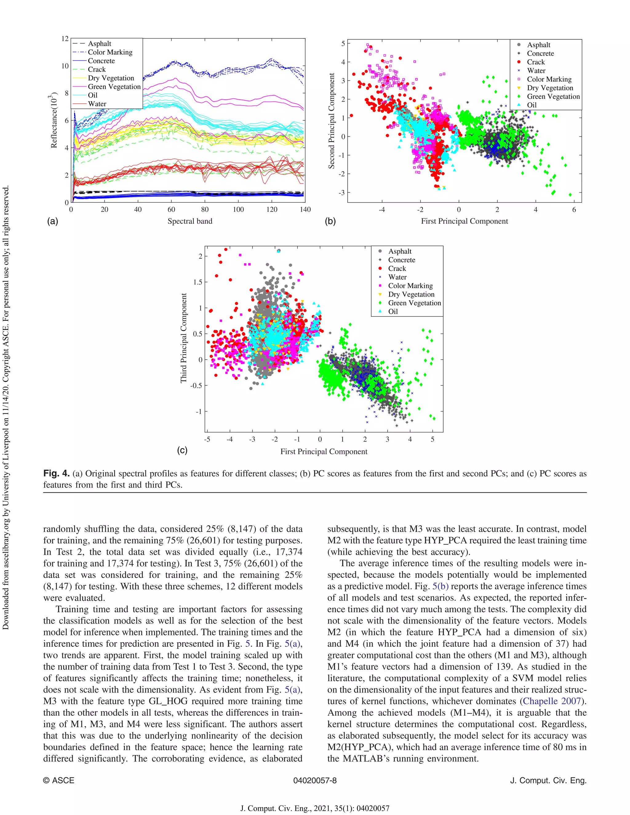
Based on the data in Eq. (3) and the original hyperspectral
pixels, three plots in Fig. 4 qualitatively illustrate the potential dis-
crimination power of hyperspectral pixels. Fig. 4(a) plots the origi-
nal spectral profiles of eight underlying objects (with only five
sample profiles for each object). Although the separability is evi-
dent, it is objectively hard to discern their potential capability of
prediction. Figs. 4(b and c) plot the first three primary PC scores
for obtained HYP_PCA features. These plotsshow the underlying
discrimination potential between all classes. HOG-based feature
vectors, which are in the form of histograms, also can be plotted;
however, it is challenging to discern their discrimination potential
visually; this is possible only through a classification model.
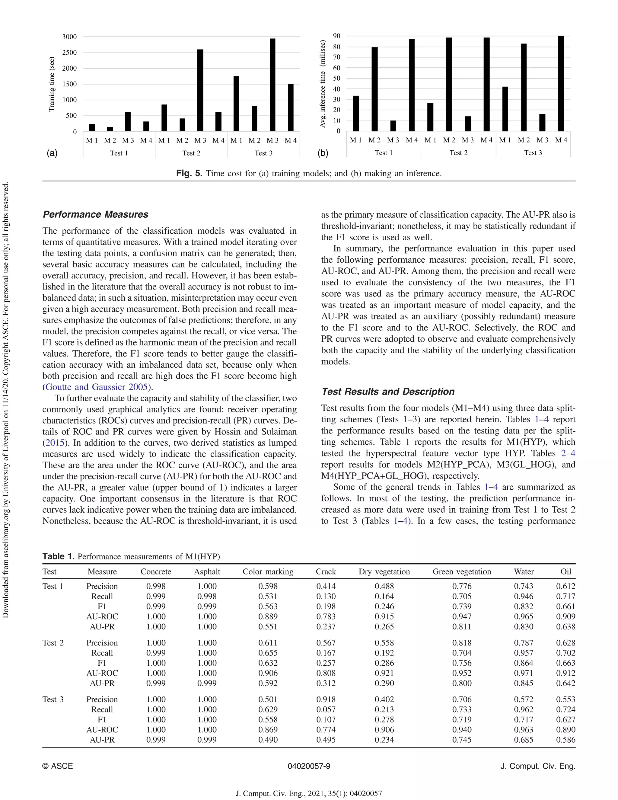
Experimental Tests and Performance Evaluation
Data Partition and Computational Cost
To proceed with the modeling and performance evaluation, a data
partition strategy is needed to split the data; one part is for the
training, and the other part is for model validation. In the literature,
the widely used scheme is to use 75% of the total data for training
and the remaining 25% for testing. Indeed, if there is a sufficient
amount of data, the data splitting ratio is flexible and is up to
the analyst. In this study, it was meaningful to examine whether
the amount of data size was sufficient, which can be determined
if the prediction performance increases with the amount of train-
ing data. Three data splitting schemes were considered for the
obtained feature data sets [Eq. (3)]. The first scheme, Test 1, after
Fig. 3. (a) Gray image of concrete surface; (b) mask image for (a); (c) gray image of asphalt surface; and (d) mask image for (c). Colored mask images
in (b) and (d) appear in the online version.
J. Comput. Civ. Eng., 2021, 35(1): 04020057
Downloaded
from
ascelibrary.org
by
University
of
Liverpool
on
11/14/20.
Copyright
ASCE.
For
personal
use
only;
all
rights
reserved.

randomly shuffling the data, considered 25% (8,147) of the data
for training, and the remaining 75% (26,601) for testing purposes.
In Test 2, the total data set was divided equally (i.e., 17,374
for training and 17,374 for testing). In Test 3, 75% (26,601) of the
data set was considered for training, and the remaining 25%
(8,147) for testing. With these three schemes, 12 different models
were evaluated.
Training time and testing are important factors for assessing
the classification models as well as for the selection of the best
model for inference when implemented. The training times and the
inference times for prediction are presented in Fig. 5. In Fig. 5(a),
two trends are apparent. First, the model training scaled up with
the number of training data from Test 1 to Test 3. Second, the type
of features significantly affects the training time; nonetheless, it
does not scale with the dimensionality. As evident from Fig. 5(a),
M3 with the feature type GL_HOG required more training time
than the other models in all tests, whereas the differences in train-
ing of M1, M3, and M4 were less significant. The authors assert
that this was due to the underlying nonlinearity of the decision
boundaries defined in the feature space; hence the learning rate
differed significantly. The corroborating evidence, as elaborated
subsequently, is that M3 was the least accurate. In contrast, model
M2 with the feature type HYP_PCA required the least training time
(while achieving the best accuracy).
The average inference times of the resulting models were in-
spected, because the models potentially would be implemented
as a predictive model. Fig. 5(b) reports the average inference times
of all models and test scenarios. As expected, the reported infer-
ence times did not vary much among the tests. The complexity did
not scale with the dimensionality of the feature vectors. Models
M2 (in which the feature HYP_PCA had a dimension of six)
and M4 (in which the joint feature had a dimension of 37) had
greater computational cost than the others (M1 and M3), although
M1’s feature vectors had a dimension of 139. As studied in the
literature, the computational complexity of a SVM model relies
on the dimensionality of the input features and their realized struc-
tures of kernel functions, whichever dominates (Chapelle 2007).
Among the achieved models (M1–M4), it is arguable that the
kernel structure determines the computational cost. Regardless,
as elaborated subsequently, the model select for its accuracy was
M2(HYP_PCA), which had an average inference time of 80 ms in
the MATLAB’s running environment.
0 20 40 60 80 100 120 140
Spectral band
0
2
4
6
8
10
12
Reflectance(10
3
)
Asphalt
Color Marking
Concrete
Crack
Dry Vegetation
Green Vegetation
Oil
Water
-4 -2 0 2 4 6
First Principal Component
-3
-2
-1
0
1
2
3
4
5
Second
Principal
Component
Asphalt
Concrete
Crack
Water
Color Marking
Dry Vegetation
Green Vegetation
Oil
-5 -4 -3 -2 -1 0 1 2 3 4 5
First Principal Component
-1
-0.5
0
0.5
1
1.5
2
Third
Principal
Component
Asphalt
Concrete
Crack
Water
Color Marking
Dry Vegetation
Green Vegetation
Oil
(a) (b)
(c)
Fig. 4. (a) Original spectral profiles as features for different classes; (b) PC scores as features from the first and second PCs; and (c) PC scores as
features from the first and third PCs.
J. Comput. Civ. Eng., 2021, 35(1): 04020057
Downloaded
from
ascelibrary.org
by
University
of
Liverpool
on
11/14/20.
Copyright
ASCE.
For
personal
use
only;
all
rights
reserved.

Performance Measures
The performance of the classification models was evaluated in
terms of quantitative measures. With a trained model iterating over
the testing data points, a confusion matrix can be generated; then,
several basic accuracy measures can be calculated, including the
overall accuracy, precision, and recall. However, it has been estab-
lished in the literature that the overall accuracy is not robust to im-
balanced data; in such a situation, misinterpretation may occur even
given a high accuracy measurement. Both precision and recall mea-
sures emphasize the outcomes of false predictions; therefore, in any
model, the precision competes against the recall, or vice versa. The
F1 score is defined as the harmonic mean of the precision and recall
values. Therefore, the F1 score tends to better gauge the classifi-
cation accuracy with an imbalanced data set, because only when
both precision and recall are high does the F1 score become high
(Goutte and Gaussier 2005).
To further evaluate the capacity and stability of the classifier, two
commonly used graphical analytics are found: receiver operating
characteristics (ROCs) curves and precision-recall (PR) curves. De-
tails of ROC and PR curves were given by Hossin and Sulaiman
(2015). In addition to the curves, two derived statistics as lumped
measures are used widely to indicate the classification capacity.
These are the area under the ROC curve (AU-ROC), and the area
under the precision-recall curve (AU-PR) for both the AU-ROC and
the AU-PR, a greater value (upper bound of 1) indicates a larger
capacity. One important consensus in the literature is that ROC
curves lack indicative power when the training data are imbalanced.
Nonetheless, because the AU-ROC is threshold-invariant, it is used
as the primary measure of classification capacity. The AU-PR also is
threshold-invariant; nonetheless, it may be statistically redundant if
the F1 score is used as well.
In summary, the performance evaluation in this paper used
the following performance measures: precision, recall, F1 score,
AU-ROC, and AU-PR. Among them, the precision and recall were
used to evaluate the consistency of the two measures, the F1
score was used as the primary accuracy measure, the AU-ROC
was treated as an important measure of model capacity, and the
AU-PR was treated as an auxiliary (possibly redundant) measure
to the F1 score and to the AU-ROC. Selectively, the ROC and
PR curves were adopted to observe and evaluate comprehensively
both the capacity and the stability of the underlying classification
models.
Test Results and Description
Test results from the four models (M1–M4) using three data split-
ting schemes (Tests 1–3) are reported herein. Tables 1–4 report
the performance results based on the testing data per the split-
ting schemes. Table 1 reports the results for M1(HYP), which
tested the hyperspectral feature vector type HYP. Tables 2–4
report results for models M2(HYP_PCA), M3(GL_HOG), and
M4(HYP_PCA+GL_HOG), respectively.
Some of the general trends in Tables 1–4 are summarized as
follows. In most of the testing, the prediction performance in-
creased as more data were used in training from Test 1 to Test 2
to Test 3 (Tables 1–4). In a few cases, the testing performance
(a) (b)
Fig. 5. Time cost for (a) training models; and (b) making an inference.
Table 1. Performance measurements of M1(HYP)
Test Measure Concrete Asphalt Color marking Crack Dry vegetation Green vegetation Water Oil
Test 1 Precision 0.998 1.000 0.598 0.414 0.488 0.776 0.743 0.612
Recall 0.999 0.998 0.531 0.130 0.164 0.705 0.946 0.717
F1 0.999 0.999 0.563 0.198 0.246 0.739 0.832 0.661
AU-ROC 1.000 1.000 0.889 0.783 0.915 0.947 0.965 0.909
AU-PR 1.000 1.000 0.551 0.237 0.265 0.811 0.830 0.638
Test 2 Precision 1.000 1.000 0.611 0.567 0.558 0.818 0.787 0.628
Recall 0.999 1.000 0.655 0.167 0.192 0.704 0.957 0.702
F1 1.000 1.000 0.632 0.257 0.286 0.756 0.864 0.663
AU-ROC 1.000 1.000 0.906 0.808 0.921 0.952 0.971 0.912
AU-PR 0.999 0.999 0.592 0.312 0.290 0.800 0.845 0.642
Test 3 Precision 1.000 1.000 0.501 0.918 0.402 0.706 0.572 0.553
Recall 1.000 1.000 0.629 0.057 0.213 0.733 0.962 0.724
F1 1.000 1.000 0.558 0.107 0.278 0.719 0.717 0.627
AU-ROC 1.000 1.000 0.869 0.774 0.906 0.940 0.963 0.890
AU-PR 0.999 0.999 0.490 0.495 0.234 0.745 0.685 0.586
J. Comput. Civ. Eng., 2021, 35(1): 04020057
Downloaded
from
ascelibrary.org
by
University
of
Liverpool
on
11/14/20.
Copyright
ASCE.
For
personal
use
only;
all
rights
reserved.

decreased in Test 3 (which used 25% of the data points for testing);
it is speculated that random shuffling occasionally may bring in
outlier data that are not learned from the training data. This obser-
vation indicates that the size of the training data does have a
positive effect on improving the accuracy of classification models.
The prediction of cracks and dry vegetation was the most challeng-
ing task. This was expected, because cracks are treated as an object
type that comes from two structural scenes (concrete and asphalt
Table 2. Performance measurements of M2(HYP_PCA)
Test 1 Precision 0.930 0.901 0.957 0.914 0.878 0.986 0.973 0.955
Recall 0.886 0.910 0.964 0.921 0.664 0.979 0.992 0.974
F1 0.907 0.906 0.961 0.917 0.757 0.982 0.983 0.964
AU-ROC 0.993 0.995 0.997 0.995 0.985 0.999 0.999 0.998
AU-PRC 0.957 0.960 0.977 0.960 0.839 0.993 0.985 0.982
Test 2 Precision 0.970 0.936 0.973 0.973 0.900 0.990 0.994 0.979
Recall 0.959 0.945 0.989 0.952 0.808 0.994 0.995 0.981
F1 0.964 0.941 0.981 0.962 0.851 0.992 0.994 0.980
AU-ROC 0.998 0.998 0.999 0.997 0.993 1.000 1.000 0.998
AU-PRC 0.987 0.983 0.985 0.987 0.893 0.995 0.997 0.985
Test 3 Precision 0.987 0.942 0.984 0.971 0.908 0.989 0.988 0.992
Recall 0.955 0.954 0.991 0.950 0.867 0.997 0.996 0.995
F1 0.971 0.948 0.988 0.960 0.887 0.993 0.992 0.993
AU-ROC 0.998 0.997 0.999 0.997 0.994 1.000 1.000 1.000
AU-PRC 0.981 0.981 0.993 0.985 0.886 0.996 0.993 0.994
Table 4. Performance measurements of M4(HYP_PCA+GL_HOG)
Test 1 Precision 0.520 0.842 0.904 0.785 0.489 0.905 0.956 0.890
Recall 0.965 0.881 0.921 0.848 0.341 0.927 0.679 0.873
F1 0.676 0.861 0.913 0.815 0.402 0.916 0.794 0.881
AU-ROC 0.978 0.992 0.993 0.985 0.938 0.993 0.974 0.986
AU-PR 0.695 0.933 0.963 0.898 0.391 0.964 0.930 0.930
Test 2 Precision 0.450 0.829 0.922 0.841 0.670 0.875 0.930 0.903
Recall 0.963 0.888 0.931 0.876 0.436 0.910 0.567 0.902
F1 0.613 0.857 0.927 0.858 0.528 0.892 0.704 0.902
AU-ROC 0.969 0.993 0.994 0.990 0.957 0.990 0.961 0.988
AU-PR 0.592 0.928 0.966 0.931 0.583 0.947 0.888 0.938
Test 3 Precision 0.779 0.761 0.931 0.895 0.779 0.947 0.969 0.925
Recall 0.939 0.962 0.935 0.835 0.529 0.951 0.851 0.894
F1 0.852 0.849 0.933 0.864 0.630 0.949 0.906 0.909
AU-ROC 0.995 0.995 0.994 0.989 0.962 0.998 0.997 0.989
AU-PR 0.946 0.957 0.970 0.924 0.683 0.985 0.981 0.944
Table 3. Performance measurements of M3(GL_HOG)
Test 1 Precision 0.560 0.580 0.723 0.575 0.724 0.740 0.888 0.725
Recall 0.559 0.598 0.781 0.195 0.234 0.731 0.943 0.845
F1 0.560 0.589 0.751 0.292 0.354 0.736 0.915 0.780
AU-ROC 0.940 0.950 0.926 0.774 0.898 0.929 0.985 0.944
AU-PR 0.549 0.615 0.724 0.295 0.365 0.750 0.932 0.764
Test 2 Precision 0.638 0.690 0.752 0.676 0.827 0.786 0.929 0.785
Recall 0.669 0.637 0.827 0.273 0.290 0.801 0.964 0.903
F1 0.653 0.662 0.788 0.389 0.430 0.793 0.946 0.840
AU-ROC 0.963 0.966 0.948 0.833 0.931 0.958 0.991 0.962
AU-PR 0.647 0.701 0.756 0.399 0.466 0.796 0.954 0.831
Test 3 Precision 0.665 0.690 0.772 0.644 0.886 0.801 0.882 0.802
Recall 0.639 0.679 0.847 0.301 0.325 0.809 0.964 0.906
F1 0.652 0.684 0.808 0.410 0.476 0.805 0.921 0.851
AU-ROC 0.959 0.969 0.942 0.828 0.948 0.962 0.990 0.964
AU-PR 0.666 0.737 0.739 0.424 0.529 0.816 0.921 0.850
J. Comput. Civ. Eng., 2021, 35(1): 04020057
Downloaded
from
ascelibrary.org
by
University
of
Liverpool
on
11/14/20.
Copyright
ASCE.
For
personal
use
only;
all
rights
reserved.

pavements), the underlying materials are very diversified, and over-
all all the reflectance intensities are darker than other objects. The
dry vegetation type had the least number of instances in the data set,
which partially contributed to the relatively poor performance com-
pared with the prediction for the green vegetation. In addition, in all
tests of all models, the precision and recall measurements were rel-
atively close for all class labels except cracks and dry vegetation.
This was particularly significant for M1(HYP) and M3(GL_HOG),
for which the recall values tended to be much smaller than the pre-
cision values. This means that in the cases of these two objects, each
instance of prediction tended to be correct; however, the models
tended to miss many objects that were either cracks or dry vegetation
objects. Furthermore, this result implies that a trade-off measure,
such as the F1 score, should be used as a better accuracy measure.
To determine the coherency and the distinction of these differ-
ent measurements, scatter plots of all measures are illustrated in
Figs. 6(a–d) for models M1–M4, respectively; for the sake of brev-
ity, only the Test 2 data scheme is included. Figs. 6(a–d) plot the F1
scores against themselves (as indicated by a 1:1 line), and all other
measurements are plotted against F1. The AU-PR as a model
capacity measure was statistically consistent with the F1 score, be-
cause it followed a linear trend in each model with a high R2 value
(R2
0.87). This implies that AU-PR largely was redundant as a
capacity measure. Therefore, the F1 score can replace it as both
a prediction accuracy measure and a model capacity measure.
The AU-ROC measure was adopted as a model-capacity measure
because it was invariant to classification thresholds and nonredun-
dant to the F1 score.
Performance Evaluation
The F1 score and AU-ROC were used as two primary performance
measures in this study. To meet the objectives outlined previously,
Figs. 7(a–d) illustrate the performance of all four models. Fig. 7(a)
shows the F1 scores for Test 1 data; Fig. 7(b) shows the F1 scores
for Test 3 data; Fig. 7(c) shows the AU-ROC for Test 1 data; and
Fig. 7(d) shows the AU-ROC for Test 3 data. The results from Test
2 are not included herein because the observed trends from Test 2
results are between Test 1 and Test 2. The following evaluation
focuses on the four objectives of this study described previously.
The F1 scores of Model M1(HYP) [Figs. 7(a and b)] indicate
that the model successfully identifies (F1 0.7) the plain concrete,
asphalt, green vegetation, and water. For the ed marking and oil, the
F1 score was about 0.6. However, for cracks and dry vegetation, the
F1 measurements were less than 0.3, indicating little prediction ac-
curacy. First, this reflects the challenge in recognizing cracks, pri-
marily caused by the inherent spectral complexity. Second, it is
primarily due to the smaller number of dry-vegetation data points.
For both objects, this presumptively is attributed to the high dimen-
sionality of the feature vectors of HYP. Nonetheless, as expected
R = 0.9882
0.1
0.3
0.5
0.7
0.9
0.1 0.3 0.5 0.7 0.9
Measure
value
F1
Preccision Recall F1
AU-ROC AU-PR Linear (F1)
Linear (AU-PR)
= 0.9181
0.8
0.85
0.9
0.95
1
0.8 0.85 0.9 0.95 1
F1
Linear (AU-PR)
= 0.9877
0.2
0.3
0.4
0.5
0.6
0.7
0.8
0.9
1
0.3 0.4 0.5 0.6 0.7 0.8 0.9 1
Measure
value
F1
Linear (AU-PR)
= 0.8724
0.4
0.5
0.6
0.7
0.8
0.9
1
0.4 0.5 0.6 0.7 0.8 0.9 1
Measure
value
F1
Linear (AU-PR)
Measure
value
2
R2
R2
R2
(a) (b)
(c) (d)
Fig. 6. Performance measurement scatter plots using Test 2 data: (a) M1; (b) M2; (c) M3; and (d) M4.
J. Comput. Civ. Eng., 2021, 35(1): 04020057
Downloaded
from
ascelibrary.org
by
University
of
Liverpool
on
11/14/20.
Copyright
ASCE.
For
personal
use
only;
all
rights
reserved.

from the AU-ROC measurements [Figs. 7(c and d)], there is no
doubt that Model M1(HYP) is highly effective in recognizing these
structural surface objects. For concrete, the average AU-ROC was
about 1. Therefore, hyperspectral pixels as feature vectors are ef-
fective in recognizing most of the structural surface objects, and
have relatively less accuracy only in the detection of cracks and
dry vegetation.
Comparing the accuracy of Model M2(HYP_PCA) with that of
M1(HYP) [Figs. 7(a and b)] showed that the detection accuracy sig-
nificantly increased. For the two weak prediction instances of cracks
and dry vegetation in M1(HYP), the F1 score increased from 0.198
to 0.917 in Test 1 and from 0.107 to 0.96 in Test 3 with Model M2
(HYP_PCA). For dry vegetation, the F1 scores changed from 0.246
to 0.757 in Test 1, and from 0.278 to 0.887 in Test 3. For all other
class labels, the classification accuracy still increased from their ini-
tially high F1 values from M1 to M2. When inspecting Fig. 7(c), the
AU-ROC measurements from M1 and M2 increased. Particularly,
the M2’s AU-ROC measurements were greater than 0.99 at predict-
ing all classes. This again signifies that Model M2(HYP_PCA) had
nearly perfect capacity to detect all structural surface objects. The
comparative tests herein provide the direct evidence that performing
dimensionality reduction over hyperspectral profiles (i.e., as HYP
feature vectors) substantially can unleash the embedded discrimina-
tion capacity of the data that otherwise is not exploitable.
A secondary yet important research problem in this work was
to prove the competitiveness of low spatial-resolution hyperspec-
tral data compared with high-resolution gray-intensity images in
detecting material surface objects. For this purpose, the results
of M2(HYP_PCA) and M3(GL_HOG) were evaluated and com-
pared. The F1 scores and the AU-ROC measurements shown in
Figs. 7(a–d), respectively, clearly indicate that in the prediction of
all class labels, M2(HYP_PCA) superseded M3(GL_HOG). Even
considering the fourth model, M4, to be evaluated, M2(HYP_PCA)
was the best model in Test 3. This model provided outstanding
performance; the smallest F1 score was 0.757, and the smallest
AU-ROC measurement was 0.985, both for predicting dry vegeta-
tion; for crack prediction, F1 ¼ 0.917 and AU-ROC ¼ 0.995. The
control model in this test, M3(GL_HOG), had F1 ¼ 0.354 and
AU-ROC ¼ 0.898 for dry vegetation, and AU-ROC ¼ 0.774, and
F1 ¼ 0.292 for cracks.
To further visualize the prediction capacity and the stability of
the two most important models in this work, M2(HYP_PCA) and
M3(GL_HOG), the ROC curves are illustrated in Figs. 8(a and b)
for the two models, respectively, based on Test 3 data. Similarly,
Figs. 9(a and b) report the PR curves. The two ROC and PR curves
show the different prediction capacity for each class label as the
underlying classification threshold changed. The ROC and PR
curves show that Model M2(HYP_PCA) had not only superb clas-
sification capability but also stronger stability, the latter of which is
indicated by the smoothness of the curves as the underlying thresh-
old varies. In the case of M3(GL_HOG), the classification capabil-
ity (and accuracy) overall was much moderate; the stability also
was worse.
For Objective 4, the authors evaluated a simple data fusion
technique, which joined the two feature types, HYP_PCA and
GL_HOG, and observed the possible performance gain or loss.
(a) (b)
(c) (d)
Fig. 7. Model performance: (a) F1 score with Test 1 data; (b) F1 score with Test 3 data; (c) AU-ROC with Test 1 data; and (d) AU-ROC with
Test 3 data.
J. Comput. Civ. Eng., 2021, 35(1): 04020057
Downloaded
from
ascelibrary.org
by
University
of
Liverpool
on
11/14/20.
Copyright
ASCE.
For
personal
use
only;
all
rights
reserved.

The comparative evaluation was conducted between M4(HYP_
PCA+GL_HOG) and M2, and between M4 and M3. In terms of
both F1 and AU-ROC measurements, the performance of M4 was
worse than that of M2. This implies that the gray value–based
features (GL_HOG) compromised the classification potential of
HYP_PCA. When M4 and M3 were assessed, for the object types
of concrete, asphalt, crack, and green vegetation, performance
increased; however, for other objects (color marking, green vegeta-
tion, water, and oil), the performance decreased.
Discussion
The observed superior performance of M2(HYP_PCA) compared
with that of M3(GL_HOG) implies that a single hyperspectral pixel
is much more effective than a 20 × 20 neighborhood of gray values
in discriminating the complex structural surface objects. Hyper-
spectral pixels with reflectance features at both visible and infrared
bands, once preprocessed (e.g., a PCA-based feature selection
step), outperformed the gray values or the embedded texture/shape
features corresponding to the hyperspectral pixel, even though the
gray images were captured at a much higher resolution (20 times
higher). Although improved gray value–based feature extraction
techniques can be used, hyperspectral pixels (which are captured
in the visible to near-infrared spectral bands with high dimension-
ality) have undoubtful promise in the detection of complex struc-
tural surface objects.
Furthermore, the methodology in this study was a traditional
machine learning paradigm. As reasoned previously, this method-
ology was proper considering the hypothesis-testing nature of this
effort. In addition, the hyperspectral data set presented in this paper
was unique, and the models developed herein form a baseline for
future studies (e.g., semantic object segmentation). Moreover, the
selected Model M2(HYP_PCA) developed herein, which is much
less complex than the latest DL models yet has very high accuracy
at pixel-level prediction, can be implemented readily in an edge-
computing device (e.g., the onboard computer that was natively
designed for the Cubert camera in our imaging system). The re-
sulting UAV-based imaging system, therefore, can realize high-
throughput hyperspectral imaging and onboard processing, in which
0 0.2 0.4 0.6 0.8 1
Recall
0
0.2
0.4
0.6
0.8
1
Precision
Concrete
Asphalt
Color Marking
Crack
Green Vegetation
Water
Oil
Dry Vegetation
0.9 0.95 1
0.8
0.85
0.9
0.95
1
0 0.1 0.2 0.3 0.4 0.5 0.6 0.7 0.8 0.9 1
Recall
0
0.1
0.2
0.3
0.4
0.5
0.6
0.7
0.8
0.9
1
Precision
Concrete
Asphalt
Color Marking
Crack
Green Vegetation
Water
Oil
Dry Vegetation
(a) (b)
Fig. 9. Precision-recall curves for (a) M2 (HYP_PCA); and (b) M3 (GL_HOG) using Test 3 data.
0 0.1 0.2 0.3 0.4 0.5 0.6 0.7 0.8 0.9 1
False positive rate
0
0.1
0.2
0.3
0.4
0.5
0.6
0.7
0.8
0.9
1
True
positive
rate
Concrete
Asphalt
Color Marking
Crack
Green Vegetation
Water
Oil
Dry Vegetation
0 0.005 0.01 0.015 0.02 0.025 0.03
0.9
0.92
0.94
0.96
0.98
1
0 0.1 0.2 0.3 0.4 0.5 0.6 0.7 0.8 0.9 1
False positive rate
0
0.1
0.2
0.3
0.4
0.5
0.6
0.7
0.8
0.9
1
True
positive
rate
Concrete
Asphalt
Color Marking
Crack
Green Vegetation
Water
Oil
Dry Vegetation
(a) (b)
Fig. 8. ROC curves for (a) M2 (HYP_PCA); and (b) M3 (GL_HOG) using Test 3 data.
J. Comput. Civ. Eng., 2021, 35(1): 04020057
Downloaded
from
ascelibrary.org
by
University
of
Liverpool
on
11/14/20.
Copyright
ASCE.
For
personal
use
only;
all
rights
reserved.

the ML model developed in this study can serve as a rapid filtering
tool so that any images with cracks (or other anomalies) can be
detected quickly. Given the resulting data filtered by the model pro-
posed in this paper, a DL model, i.e., a semantic spatial-spectral
segmentation model, can be deployed to realize more detailed
and semantics-rich damage detection.
One specific future direction is to extract spectral–spatial fea-
tures using a more integral approach. As mentioned previously, a
pansharpening technique can be used to generate a high spatial-
resolution hyperspectral cube. Specifically, the hyperspectral cube
of 20 × 20 × 139 used in this study can be turned into a cube
with much higher spatial dimension, namely a 1,000 × 1,000 ×
139 cube. With this 3D cube, and a mask image of the same size,
advanced spatial-spectral features may be extracted (Fang et al.
2018; Hang et al. 2015; Zhang et al. 2014), and then a classifier
(e.g., a kernel SVM as used in this study) can be adopted. This
pansharpening may act as an effective data augmentation tech-
nique, such that it can support a deep learning architecture. This
promising direction is beyond the scope of this work.
Conclusion
A mobile hyperspectral imaging system was developed for ground-
based and aerial data collection. One of its primary applications
is to inspect surfaces of structural materials, such as concrete and
asphalt materials, which commonly are used in transportation struc-
tures. The innovation lies in its ability to detect surface damage
and other artifacts at the material levels due to its high-dimensional
pixels with reflectance in both visible and near-infrared bands. The
effectiveness of the technique was proven in composition with
regular gray-level images that are very high-resolution and com-
monly used in practice. Four machine-learning models character-
ized by different feature description processes were trained and
tested. With a total of 34,748 labeled features of different types,
three data-splitting schemes were used to evaluate the effects of
data size. A multiclass support vector machine with a Gaussian
kernel was adopted in all models. State-of-the-art measures were
adopted to test the models, and the issue of data imbalance was
considered. From a comprehensive evaluation, two major conclu-
sions were formulated:
1. The use of hyperspectral reflectance values at pixels as feature
vectors was effective in recognizing all eight surface objects.
However, dimensionality reduction is essential for this effective-
ness. The linear PCA approach was adopted; using only the first
six component scores, the resulting classification models were
highly accurate, high-capacity, and stable.
2. Compared with the model based on gray-level features (GL_
HOG), based on a popular variant of the HOG descriptor, the
PCA-adapted hyperspectral features had much better detection
performance. A single hyperspectral pixel with high-dimension
spectral reflectance evidentially is competitive compared with
the corresponding high-resolution gray intensities that express
the shape and texture of the underlying objects. The data fusion
technique in this study had a less desirable performance, which
may be due to the simple concatenation technique used to
combine the GL_HOG and HYP_PCA features.
With the experimental and machine learning–based evaluation
results in this paper, the authors further envision the dawn of com-
putational hyperspectral imaging or hyperspectral machine vision
for material damage detection in civil engineering and their promise
in dealing with complex scenes that are often found in civil struc-
tures in service.
Data Availability Statement
Some or all data, models, or code generated or used during the
study are available from the corresponding author by request.
The training and testing data set is archived publicly (Chen 2020).
Acknowledgments
This material is based partially upon work supported by the National
Science Foundation (NSF) under Award number No. IIA-1355406
and work supported by the United States Department of Agricul-
ture’s National Institute of Food and Agriculture (USDA-NIFA)
under Award No. 2015-68007-23214. Any opinions, findings, and
conclusions or recommendations expressed in this material are those
of the author(s) and do not necessarily reflect the views of NSF or
USDA-NIFA.
References
AASHTO. 2019. Manual for bridge element inspection. Washington, DC:
AASHTO.
Adler-Golden, S., A. Berk, L. Bernstein, S. Richtsmeier, P. Acharya, M.
Matthew, G. Anderson, C. Allred, L. Jeong, and J. Chetwynd. 1998.
“FLAASH, a MODTRAN4 atmospheric correction package for hyper-
spectral data retrievals and simulations.” In Proc., 7th JPL Airborne
Earth Science Workshop, 9–14. Pasadena, CA: California Institute
of Technology.
Alipour, M., D. K. Harris, and G. R. Miller. 2019. “Robust pixel-level crack
detection using deep fully convolutional neural networks.” J. Comput.
Civ. Eng. 33 (6): 04019040. https://doi.org/10.1061/(ASCE)CP.1943
-5487.0000854.
Bandos, T. V., L. Bruzzone, and G. Camps-Valls. 2009. “Classification of
hyperspectral images with regularized linear discriminant analysis.”
IEEE Trans. Geosci. Remote Sens. 47 (3): 862–873. https://doi.org/10
.1109/TGRS.2008.2005729.
Baumgardner, M. F., L. L. Biehl, and D. A. Landgrebe. 2015. 220 band
AVIRIS hyperspectral image data set: June 12, 1992 Indian Pine Test
Site 3. West Lafayette, IN: Purdue Univ. Research Repository. https://
doi.org/10.4231/R7RX991C.
Bilal, M., and M. S. Hanif. 2020. “Benchmark revision for HOG-SVM
pedestrian detector through reinvigorated training and evaluation meth-
odologies.” IEEE Trans. Intell. Transp. Syst. 21 (3): 1277–1287. https://
doi.org/10.1109/TITS.2019.2906132.
Bioucas-Dias, J. M., A. Plaza, N. Dobigeon, M. Parente, Q. Du, P. Gader,
and J. Chanussot. 2012. “Hyperspectral unmixing overview: Geomet-
rical, statistical, and sparse regression-based approaches.” IEEE J. Sel.
Top. Appl. Earth Obs. Remote Sens. 5 (2): 354–379. https://doi.org/10
.1109/JSTARS.2012.2194696.
Bodkin, A., A. Sheinis, A. Norton, J. Daly, S. Beaven, and J. Weinheimer.
2009. “Snapshot hyperspectral imaging: The hyperpixel array camera.”
In Proc., Algorithms and Technologies for Multispectral, Hyperspec-
tral, and Ultraspectral Imagery XV, 73340H. Bellingham, WA:
International Society for Optics and Photonics.
Bristow, H., and S. Lucey. 2014. Why do linear SVMs trained on HOG
features perform so well? Ithaca, NY: Cornell Univ.
Cawley, P. 2018. “Structural health monitoring: Closing the gap between
research and industrial deployment.” Struct. Health Monit. 17 (5):
1225–1244. https://doi.org/10.1177/1475921717750047.
Cha, Y.-J., W. Choi, and O. Büyüköztürk. 2017. “Deep learning-based crack
damage detection using convolutional neural networks.” Comput.-Aided
Civ. Infrastruct. Eng. 32 (5): 361–378. https://doi.org/10.1111/mice
.12263.
Chapelle, O. 2007. “Training a support vector machine in the primal.”
Neural Comput. 19 (5): 1155–1178. https://doi.org/10.1162/neco.2007
.19.5.1155.
J. Comput. Civ. Eng., 2021, 35(1): 04020057
Downloaded
from
ascelibrary.org
by
University
of
Liverpool
on
11/14/20.
Copyright
ASCE.
For
personal
use
only;
all
rights
reserved.

Chen, G., and S.-E. Qian. 2007. “Dimensionality reduction of hyperspectral
imagery.” J. Appl. Remote Sens. 1 (1): 013509. https://doi.org/10.1117
/1.2723663.
Chen, G., and S.-E. Qian. 2008. “Simultaneous dimensionality reduction
and denoising of hyperspectral imagery using bivariate wavelet shrink-
ing and principal component analysis.” Can. J. Remote Sens. 34 (5):
447–454. https://doi.org/10.5589/m08-058.
Chen, Y., H. Jiang, C. Li, X. Jia, and P. Ghamisi. 2016. “Deep feature ex-
traction and classification of hyperspectral images based on convolu-
tional neural networks.” IEEE Trans. Geosci. Remote Sens. 54 (10):
6232–6251. https://doi.org/10.1109/TGRS.2016.2584107.
Chen, Y., Z. Lin, X. Zhao, G. Wang, and Y. Gu. 2014. “Deep learning-
based classification of hyperspectral data.” IEEE J. Sel. Top. Appl.
Earth Obs. Remote Sens. 7 (6): 2094–2107. https://doi.org/10.1109
/JSTARS.2014.2329330.
Chen, Z. 2020. “Hyperspectral imagery for material surface damage.” Fig-
share. https://doi.org/10.6084/m9.figshare.12385994.v1.
Chen, Z., J. Chen, F. Shen, and Y. Lee. 2015. “Collaborative mobile-cloud
computing for civil infrastructure condition inspection.” J. Comput. Civ.
Eng. 29 (5): 04014066. https://doi.org/10.1061/(ASCE)CP.1943-5487
.0000377.
Chen, Z., R. Derakhshani, C. Halmen, and J. T. Kevern. 2011. “A texture-
based method for classifying cracked concrete surfaces from digital im-
ages using neural networks.” In Proc., 2011 Int. Joint Conf. on Neural
Networks, 2632–2637. New York: IEEE.
Chen, Z., and T. C. Hutchinson. 2010. “Image-based framework for
concrete surface crack monitoring and quantification.” Adv. Civ. Eng.
2010: 215295. https://doi.org/10.1155/2010/215295.
Cheng, H. D., and M. Miyojim. 1998. “Automatic pavement distress
detection system.” Inf. Sci. 108 (1): 219–240. https://doi.org/10.1016
/S0020-0255(97)10062-7.
Cooley, T., et al. 2002.“FLAASH, a MODTRAN4-based atmospheric
correction algorithm, its application and validation.” In Proc., IEEE
Int. Geoscience and Remote Sensing Symp., 1414–1418. New York:
IEEE.
Cubert. 2018. “Hyperspectral VNIR Camera FireflEYE 185.” Accessed
January 1, 2020. https://cubert-gmbh.com/product/firefleye-185
-hyperspectral/.
Dalal, N., and B. Triggs. 2005.“Histograms of oriented gradients for human
detection.” In Vol. 881 of Proc., IEEE Computer Society Conf. on
Computer Vision and Pattern Recognition (CVPR’05), 886–893.
New York: IEEE.
Duan, K.-B., J. C. Rajapakse, and M. N. Nguyen. 2007. “One-versus-one
and one-versus-all multiclass SVM-RFE for gene selection in cancer
classification.” In Proc., Evolutionary Computation, Machine Learning
and Data Mining in Bioinformatics, 47–56. Berlin: Springer.
Fang, L., N. He, S. Li, A. J. Plaza, and J. Plaza. 2018. “A new spatial–
spectral feature extraction method for hyperspectral images using local
covariance matrix representation.” IEEE Trans. Geosci. Remote Sens.
56 (6): 3534–3546. https://doi.org/10.1109/TGRS.2018.2801387.
Felzenszwalb, P. F., R. B. Girshick, D. McAllester, and D. Ramanan. 2010.
“Object detection with discriminatively trained part-based models.”
IEEE Trans. Pattern Anal. Mach. Intell. 32 (9): 1627–1645. https://doi
.org/10.1109/TPAMI.2009.167.
Foody, G. M., and A. Mathur. 2006. “The use of small training sets con-
taining mixed pixels for accurate hard image classification: Training on
mixed spectral responses for classification by a SVM.” Remote Sens.
Environ. 103 (2): 179–189. https://doi.org/10.1016/j.rse.2006.04.001.
Gavilán, M., D. Balcones, O. Marcos, D. F. Llorca, M. A. Sotelo, I. Parra,
M. Ocaña, P. Aliseda, P. Yarza, and A. Amírola. 2011. “Adaptive road
crack detection system by pavement classification.” Sensors 11 (10):
9628–9657. https://doi.org/10.3390/s111009628.
Goel, P. K., S. O. Prasher, R. M. Patel, J. A. Landry, R. B. Bonnell, and
A. A. Viau. 2003. “Classification of hyperspectral data by decision trees
and artificial neural networks to identify weed stress and nitrogen status
of corn.” Comput. Electron. Agric. 39 (2): 67–93. https://doi.org/10
.1016/S0168-1699(03)00020-6.
Goutte, C., and E. Gaussier. 2005. “A probabilistic interpretation of
precision, recall and F-score, with implication for evaluation.” In Proc.,
European Conf. on Information Retrieval, 345–359. New York:
Springer.
Graña, M., M. Veganzons, and B. Ayerdi. 2020. “Hyperspectral remote
sensing scenes.” Accessed May 1, 2020. http://www.ehu.eus/ccwintco
/index.php/Hyperspectral_Remote_Sensing_Scenes.
Green, R. O., et al. 1998. “Imaging spectroscopy and the airborne visible/
infrared imaging spectrometer (AVIRIS).” Remote Sens. Environ.
65 (3): 227–248. https://doi.org/10.1016/S0034-4257(98)00064-9.
Hang, R., Q. Liu, H. Song, and Y. Sun. 2015. “Matrix-based discriminant
subspace ensemble for hyperspectral image spatial–spectral feature fu-
sion.” IEEE Trans. Geosci. Remote Sens. 54 (2): 783–794. https://doi
.org/10.1109/TGRS.2015.2465899.
Hang, R., Q. Liu, Y. Sun, X. Yuan, H. Pei, J. Plaza, and A. Plaza. 2017.
“Robust matrix discriminative analysis for feature extraction from hy-
perspectral images.” IEEE J. Sel. Top. Appl. Earth Obs. Remote Sens.
10 (5): 2002–2011. https://doi.org/10.1109/JSTARS.2017.2658948.
Harsanyi, J. C., and C. Chang. 1994. “Hyperspectral image classification
and dimensionality reduction: an orthogonal subspace projection ap-
proach.” IEEE Trans. Geosci. Remote Sens. 32 (4): 779–785. https://doi
.org/10.1109/36.298007.
Heylen, R., M. Parente, and P. Gader. 2014. “A review of nonlinear
hyperspectral unmixing methods.” IEEE J. Sel. Top. Appl. Earth
Obs. Remote Sens. 7 (6): 1844–1868. https://doi.org/10.1109/JSTARS
.2014.2320576.
Ho, H.-N., K.-D. Kim, Y.-S. Park, and J.-J. Lee. 2013. “An efficient image-
based damage detection for cable surface in cable-stayed bridges.” NDT
E Int. 58 (Sep): 18–23. https://doi.org/10.1016/j.ndteint.2013.04.006.
Hossin, M., and M. N. Sulaiman. 2015. “A review on evaluation metrics
for data classification evaluations.” Int. J. Data Min. Knowl. Manage.
Process 5 (2): 1. https://doi.org/10.5121/ijdkp.2015.5201.
Hu, W., and C. Jia. 2015. “A bootstrapping approach to entity linkage on
the semantic web.” J. Web Semant. 34 (Oct): 1–12. https://doi.org/10
.1016/j.websem.2015.07.003.
Isawa, K., S. Nakayama, M. Ikeda, S. Takagi, S. Tosaka, and N. Kasai.
2005. “Robotic 3D SQUID imaging system for practical nondestructive
evaluation applications.” Physica C 432 (3–4): 182–192. https://doi.org
/10.1016/j.physc.2005.08.008.
Ji, R., Y. Gao, R. Hong, Q. Liu, D. Tao, and X. Li. 2014. “Spectral-spatial
constraint hyperspectral image classification.” IEEE Trans. Geosci.
Remote Sens. 52 (3): 1811–1824. https://doi.org/10.1109/TGRS.2013
.2255297.
Johnson, W. R., D. W. Wilson, G. H. Bearman, and J. Backlund. 2004. “An
all-reflective computed tomography imaging spectrometer.” In Proc.,
Instruments, Science, and Methods for Geospace and Planetary Remote
Sensing, 88–97. Bellingham, WA: International Society for Optics and
Photonics.
Kaiser, P. K., and R. M. Boynton. 1996. Human color vision. Washington,
DC: Optical Society of America.
Kaseko, M. S., and S. G. Ritchie. 1993. “A neural network-based method-
ology for pavement crack detection and classification.” Transp. Res.
Part C: Emerging Technol. 1 (4): 275–291. https://doi.org/10.1016
/0968-090X(93)90002-W.
Kim, H., S. Sim, and S. Cho. 2015. “Unmanned aerial vehicle (UAV)-
powered concrete crack detection based on digital image processing.”
In Proc., Int. Conf. on Advances in Experimental Structural Engineer-
ing. Urbana-Champaign, IL: Univ. of Illinois.
Lattanzi, D. A., and G. Miller. 2013. “A prototype imaging and visualiza-
tion system for robotic infrastructure inspection.” In Proc., Structures
Congress 2013: Bridging Your Passion with Your Profession, 410–421.
Reston, VA: ASCE.
Leshko, B. J. 2002. Guidelines for inspecting complex components of
bridges. Washington, DC: AASHTO.
Li, W., G. Wu, F. Zhang, and Q. Du. 2017. “Hyperspectral image classi-
fication using deep pixel-pair features.” IEEE Trans. Geosci. Remote
Sens. 55 (2): 844–853. https://doi.org/10.1109/TGRS.2016.2616355.
Liu, Z., S. A. Suandi, T. Ohashi, and T. Ejima. 2002.“Tunnel crack detec-
tion and classification system based on image processing.” In Proc.,
Machine Vision Applications in Industrial Inspection X, 145–152. Bel-
lingham, WA: International Society for Optics and Photonics.
J. Comput. Civ. Eng., 2021, 35(1): 04020057
Downloaded
from
ascelibrary.org
by
University
of
Liverpool
on
11/14/20.
Copyright
ASCE.
For
personal
use
only;
all
rights
reserved.

Loncan, L., L. B. De Almeida, J. M. Bioucas-Dias, X. Briottet,
J. Chanussot, N. Dobigeon, S. Fabre, W. Liao, G. A. Licciardi, and
M. Simoes. 2015. “Hyperspectral pansharpening: A review.” IEEE
Geosci. Remote Sens. Mag. 3 (3): 27–46. https://doi.org/10.1109/MGRS
.2015.2440094.
Lu, G., and B. Fei. 2014. “Medical hyperspectral imaging: A review.”
J. Biomed. Opt. 19 (1): 010901. https://doi.org/10.1117/1.JBO.19.1
.010901.
Marpu, P. R., P. Gamba, and I. Niemeyer. 2009. “Hyperspectral data
classification using an ensemble of class-dependent neural networks.”
In Proc., 2009 1st Workshop on Hyperspectral Image and Signal
Processing: Evolution in Remote Sensing, 1–4. New York: IEEE.
Mercier, G., and M. Lennon. 2003. “Support vector machines for hyper-
spectral image classification with spectral-based kernels.” In Vol. 281 of
Proc., IGARSS 2003. 2003 IEEE Int. Geoscience and Remote Sensing
Symp. (IEEE Cat. No.03CH37477), 288–290. New York: IEEE.
Morris, T. 2004. Computer vision and image processing. Basingstoke, UK:
Palgrave Macmillan.
Ni, F., J. Zhang, and Z. Chen. 2019. “Pixel-level crack delineation in
images with convolutional feature fusion.” Struct. Control Health
Monit. 26 (1): e2286. https://doi.org/10.1002/stc.2286.
Olsen, M. J., A. Barbosa, P. Burns, A. Kashani, H. Wang, M. Veletzos,
Z. Chen, G. Roe, and K. Tabrizi. 2016. Assessing, coding, and marking
of highway structures in emergency situations, Volume 1: Research
overview. Washington, DC: Transportation Research Board.
Ozer, E., M. Q. Feng, and D. Feng. 2015. “Citizen sensors for SHM:
Towards a crowdsourcing platform.” Sensors 15 (6): 14591–14614.
https://doi.org/10.3390/s150614591.
Palsson, F., J. R. Sveinsson, M. O. Ulfarsson, and J. A. Benediktsson. 2015.
“Model-based fusion of multi- and hyperspectral images using PCA and
wavelets.” IEEE Trans. Geosci. Remote Sens. 53 (5): 2652–2663.
https://doi.org/10.1109/TGRS.2014.2363477.
Plaza, A., et al. 2009. “Recent advances in techniques for hyperspectral
image processing.” Remote Sens. Environ. Supplement, 113 (S1):
S110–S122. https://doi.org/10.1016/j.rse.2007.07.028.
Prasanna, P., K. J. Dana, N. Gucunski, B. B. Basily, H. M. La, R. S. Lim,
and H. Parvardeh. 2014. “Automated crack detection on concrete
bridges.” IEEE Trans. Autom. Sci. Eng. 13 (2): 591–599. https://doi
.org/10.1109/TASE.2014.2354314.
Ritchie, S. G. 1987. “Expert systems in pavement management.” Transp.
Res. Part A: General 21 (2): 145–152. https://doi.org/10.1016/0191
-2607(87)90007-0.
Ritchie, S. G. 1990. “Digital imaging concepts and applications in pave-
ment management.” J. Transp. Eng. 116 (3): 287–298. https://doi.org
/10.1061/(ASCE)0733-947X(1990)116:3(287).
Roh, Y., G. Heo, and S. E. Whang. 2019. “A survey on data collection for
machine learning: A big data—AI integration perspective.” In Proc.,
IEEE Transactions on Knowledge and Data Engineering. New York:
IEEE.
Siesler, H. W., Y. Ozaki, S. Kawata, and H. M. Heise. 2008. Near-infrared
spectroscopy: Principles, instruments, applications. New York: Wiley.
Sohn, H., C. R. Farrar, F. M. Hemez, D. D. Shunk, D. W. Stinemates, B. R.
Nadler, and J. J. Czarnecki. 2003. A review of structural health mon-
itoring literature: 1996–2001. Los Alamos, NM: Los Alamos National
Laboratory.
Tang S., and Z. Chen. 2017. “Detection of complex concrete damage—A
deep learning framework and performance evaluation.” In Int. Work-
shop on Computing for Civil Engineering (IWCCE). Seattle, WA:
ASCE.
Tung, P.-C., Y.-R. Hwang, and M.-C. Wu. 2002. “The development of
a mobile manipulator imaging system for bridge crack inspection.”
Autom. Constr. 11 (6): 717–729. https://doi.org/10.1016/S0926-5805
(02)00012-2.
Yeum, C. M., and S. J. Dyke. 2015. “Vision-based automated crack detec-
tion for bridge inspection.” Comput.-Aided Civ. Infrastruct. Eng.
30 (10): 759–770. https://doi.org/10.1111/mice.12141.
Zakeri, H., F. M. Nejad, and A. Fahimifar. 2017. “Image based techniques
for crack detection, classification and quantification in asphalt pave-
ment: A review.” Arch. Comput. Methods Eng. 24 (4): 935–977. https://
doi.org/10.1007/s11831-016-9194-z.
Zhang, C., and A. Elaksher. 2012. “An unmanned aerial vehicle-based im-
aging system for 3D measurement of unpaved road surface distresses.”
Comput.-Aided Civ. Infrastruct. Eng. 27 (2): 118–129. https://doi.org
/10.1111/j.1467-8667.2011.00727.x.
Zhang, L., F. Yang, Y. D. Zhang, and Y. J. Zhu. 2016. “Road crack
detection using deep convolutional neural network.” In Proc., 2016
IEEE Int. Conf. on Image Processing (ICIP), 3708–3712. New York:
IEEE.
Zhang, Q., Y. Tian, Y. Yang, and C. Pan. 2014. “Automatic spatial–spectral
feature selection for hyperspectral image via discriminative sparse mul-
timodal learning.” IEEE Trans. Geosci. Remote Sens. 53 (1): 261–279.
https://doi.org/10.1109/TGRS.2014.2321405.
J. Comput. Civ. Eng., 2021, 35(1): 04020057
Downloaded
from
ascelibrary.org
by
University
of
Liverpool
on
11/14/20.
Copyright
ASCE.
For
personal
use
only;
all
rights
reserved.

Aryal.pdf

Recommended

Recommended

More Related Content

Similar to Aryal.pdf

Similar to Aryal.pdf (20)

More from PreetiKulkarni20

More from PreetiKulkarni20 (8)

Recently uploaded

Recently uploaded (20)

Aryal.pdf