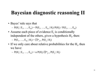
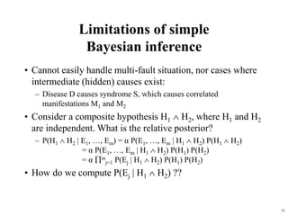
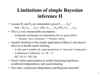
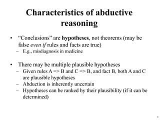
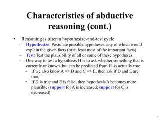
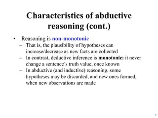
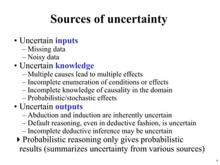
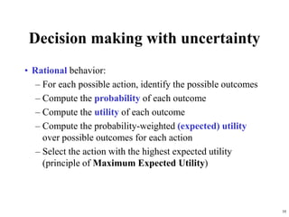
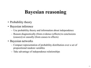
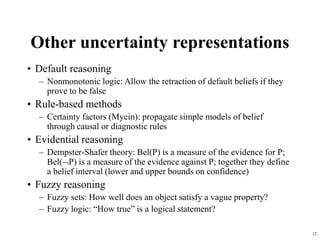
This document discusses abductive reasoning, focusing on its differences from deduction and induction, and emphasizes the inherent uncertainty in forming plausible explanations for observations. It reviews various formalisms for representing uncertainty, such as Bayesian networks and Dempster-Shafer theory, and highlights decision-making strategies under uncertainty. The document also covers the limitations and applications of Bayesian reasoning in diagnostic contexts.

1. 1
Knowledge
Representation and
Reasoning
Chapter 10.1-10.2, 10.6
CS 63
Adapted from slides by
Tim Finin and
Marie desJardins.
Some material adopted from notes
by Andreas Geyer-Schulz,
and Chuck Dyer.

2. 2
Abduction
• Abduction is a reasoning process that tries to form plausible
explanations for abnormal observations
– Abduction is distinctly different from deduction and induction
– Abduction is inherently uncertain
• Uncertainty is an important issue in abductive reasoning
• Some major formalisms for representing and reasoning about
uncertainty
– Mycin’s certainty factors (an early representative)
– Probability theory (esp. Bayesian belief networks)
– Dempster-Shafer theory
– Fuzzy logic
– Truth maintenance systems
– Nonmonotonic reasoning

3. 3
Abduction
• Definition (Encyclopedia Britannica): reasoning that derives
an explanatory hypothesis from a given set of facts
– The inference result is a hypothesis that, if true, could
explain the occurrence of the given facts
• Examples
– Dendral, an expert system to construct 3D structure of
chemical compounds
• Fact: mass spectrometer data of the compound and its
chemical formula
• KB: chemistry, esp. strength of different types of bounds
• Reasoning: form a hypothetical 3D structure that satisfies the
chemical formula, and that would most likely produce the
given mass spectrum

4. 4
– Medical diagnosis
• Facts: symptoms, lab test results, and other observed findings
(called manifestations)
• KB: causal associations between diseases and manifestations
• Reasoning: one or more diseases whose presence would
causally explain the occurrence of the given manifestations
– Many other reasoning processes (e.g., word sense
disambiguation in natural language process, image
understanding, criminal investigation) can also been seen
as abductive reasoning
Abduction examples (cont.)

5. 5
Comparing abduction, deduction,
and induction
Deduction: major premise: All balls in the box are black
minor premise: These balls are from the box
conclusion: These balls are black
Abduction: rule: All balls in the box are black
observation: These balls are black
explanation: These balls are from the box
Induction: case: These balls are from the box
observation: These balls are black
hypothesized rule: All ball in the box are black
A => B
A
---------
B
A => B
B
-------------
Possibly A
Whenever
A then B
-------------
Possibly
A => B
Deduction reasons from causes to effects
Abduction reasons from effects to causes
Induction reasons from specific cases to general rules

6. 6
Characteristics of abductive
reasoning
• “Conclusions” are hypotheses, not theorems (may be
false even if rules and facts are true)
– E.g., misdiagnosis in medicine
• There may be multiple plausible hypotheses
– Given rules A => B and C => B, and fact B, both A and C
are plausible hypotheses
– Abduction is inherently uncertain
– Hypotheses can be ranked by their plausibility (if it can be
determined)

7. 7
Characteristics of abductive
reasoning (cont.)
• Reasoning is often a hypothesize-and-test cycle
– Hypothesize: Postulate possible hypotheses, any of which would
explain the given facts (or at least most of the important facts)
– Test: Test the plausibility of all or some of these hypotheses
– One way to test a hypothesis H is to ask whether something that is
currently unknown–but can be predicted from H–is actually true
• If we also know A => D and C => E, then ask if D and E are
true
• If D is true and E is false, then hypothesis A becomes more
plausible (support for A is increased; support for C is
decreased)

8. 8
Characteristics of abductive
reasoning (cont.)
• Reasoning is non-monotonic
– That is, the plausibility of hypotheses can
increase/decrease as new facts are collected
– In contrast, deductive inference is monotonic: it never
change a sentence’s truth value, once known
– In abductive (and inductive) reasoning, some
hypotheses may be discarded, and new ones formed,
when new observations are made

9. 9
Sources of uncertainty
• Uncertain inputs
– Missing data
– Noisy data
• Uncertain knowledge
– Multiple causes lead to multiple effects
– Incomplete enumeration of conditions or effects
– Incomplete knowledge of causality in the domain
– Probabilistic/stochastic effects
• Uncertain outputs
– Abduction and induction are inherently uncertain
– Default reasoning, even in deductive fashion, is uncertain
– Incomplete deductive inference may be uncertain
Probabilistic reasoning only gives probabilistic
results (summarizes uncertainty from various sources)

10. 10
Decision making with uncertainty
• Rational behavior:
– For each possible action, identify the possible outcomes
– Compute the probability of each outcome
– Compute the utility of each outcome
– Compute the probability-weighted (expected) utility
over possible outcomes for each action
– Select the action with the highest expected utility
(principle of Maximum Expected Utility)

11. 11
Bayesian reasoning
• Probability theory
• Bayesian inference
– Use probability theory and information about independence
– Reason diagnostically (from evidence (effects) to conclusions
(causes)) or causally (from causes to effects)
• Bayesian networks
– Compact representation of probability distribution over a set of
propositional random variables
– Take advantage of independence relationships

12. 12
Other uncertainty representations
• Default reasoning
– Nonmonotonic logic: Allow the retraction of default beliefs if they
prove to be false
• Rule-based methods
– Certainty factors (Mycin): propagate simple models of belief
through causal or diagnostic rules
• Evidential reasoning
– Dempster-Shafer theory: Bel(P) is a measure of the evidence for P;
Bel(P) is a measure of the evidence against P; together they define
a belief interval (lower and upper bounds on confidence)
• Fuzzy reasoning
– Fuzzy sets: How well does an object satisfy a vague property?
– Fuzzy logic: “How true” is a logical statement?

13. 13
Uncertainty tradeoffs
• Bayesian networks: Nice theoretical properties combined
with efficient reasoning make BNs very popular; limited
expressiveness, knowledge engineering challenges may
limit uses
• Nonmonotonic logic: Represent commonsense reasoning,
but can be computationally very expensive
• Certainty factors: Not semantically well founded
• Dempster-Shafer theory: Has nice formal properties, but
can be computationally expensive, and intervals tend to
grow towards [0,1] (not a very useful conclusion)
• Fuzzy reasoning: Semantics are unclear (fuzzy!), but has
proved very useful for commercial applications

14. 14
Bayesian Reasoning
Chapter 13
CS 63
Adapted from slides by
Tim Finin and
Marie desJardins.

15. 15
Outline
• Probability theory
• Bayesian inference
– From the joint distribution
– Using independence/factoring
– From sources of evidence

16. 16
Sources of uncertainty
• Uncertain inputs
– Missing data
– Noisy data
• Uncertain knowledge
– Multiple causes lead to multiple effects
– Incomplete enumeration of conditions or effects
– Incomplete knowledge of causality in the domain
– Probabilistic/stochastic effects
• Uncertain outputs
– Abduction and induction are inherently uncertain
– Default reasoning, even in deductive fashion, is uncertain
– Incomplete deductive inference may be uncertain
Probabilistic reasoning only gives probabilistic
results (summarizes uncertainty from various sources)

17. 17
Decision making with uncertainty
• Rational behavior:
– For each possible action, identify the possible outcomes
– Compute the probability of each outcome
– Compute the utility of each outcome
– Compute the probability-weighted (expected) utility
over possible outcomes for each action
– Select the action with the highest expected utility
(principle of Maximum Expected Utility)

18. 18
Why probabilities anyway?
• Kolmogorov showed that three simple axioms lead to the
rules of probability theory
– De Finetti, Cox, and Carnap have also provided compelling
arguments for these axioms
1. All probabilities are between 0 and 1:
• 0 ≤ P(a) ≤ 1
2. Valid propositions (tautologies) have probability 1, and
unsatisfiable propositions have probability 0:
• P(true) = 1 ; P(false) = 0
3. The probability of a disjunction is given by:
• P(a  b) = P(a) + P(b) – P(a  b)
ab
a b

19. 19
Probability theory
• Random variables
– Domain
• Atomic event: complete
specification of state
• Prior probability: degree
of belief without any other
evidence
• Joint probability: matrix
of combined probabilities
of a set of variables
• Alarm, Burglary, Earthquake
– Boolean (like these), discrete,
continuous
• (Alarm=True  Burglary=True 
Earthquake=False) or equivalently
(alarm  burglary  ¬earthquake)
• P(Burglary) = 0.1
• P(Alarm, Burglary) =
alarm ¬alarm
burglary 0.09 0.01
¬burglary 0.1 0.8

20. 20
Probability theory (cont.)
• Conditional probability:
probability of effect given causes
• Computing conditional probs:
– P(a | b) = P(a  b) / P(b)
– P(b): normalizing constant
• Product rule:
– P(a  b) = P(a | b) P(b)
• Marginalizing:
– P(B) = ΣaP(B, a)
– P(B) = ΣaP(B | a) P(a)
(conditioning)
• P(burglary | alarm) = 0.47
P(alarm | burglary) = 0.9
• P(burglary | alarm) =
P(burglary  alarm) / P(alarm)
= 0.09 / 0.19 = 0.47
• P(burglary  alarm) =
P(burglary | alarm) P(alarm) =
0.47 * 0.19 = 0.09
• P(alarm) =
P(alarm  burglary) +
P(alarm  ¬burglary) =
0.09 + 0.1 = 0.19

21. 21
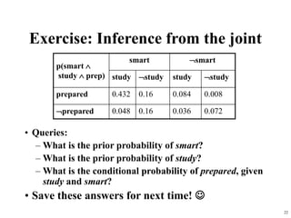
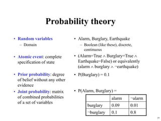
Example: Inference from the joint
alarm ¬alarm
earthquake ¬earthquake earthquake ¬earthquake
burglary 0.01 0.08 0.001 0.009
¬burglary 0.01 0.09 0.01 0.79
P(Burglary | alarm) = α P(Burglary, alarm)
= α [P(Burglary, alarm, earthquake) + P(Burglary, alarm, ¬earthquake)
= α [ (0.01, 0.01) + (0.08, 0.09) ]
= α [ (0.09, 0.1) ]
Since P(burglary | alarm) + P(¬burglary | alarm) = 1, α = 1/(0.09+0.1) = 5.26
(i.e., P(alarm) = 1/α = 0.109 Quizlet: how can you verify this?)
P(burglary | alarm) = 0.09 * 5.26 = 0.474
P(¬burglary | alarm) = 0.1 * 5.26 = 0.526

22. 22
Exercise: Inference from the joint
• Queries:
– What is the prior probability of smart?
– What is the prior probability of study?
– What is the conditional probability of prepared, given
study and smart?
• Save these answers for next time! 
p(smart 
study  prep)
smart smart
study study study study
prepared 0.432 0.16 0.084 0.008
prepared 0.048 0.16 0.036 0.072

23. 23
Independence
• When two sets of propositions do not affect each others’
probabilities, we call them independent, and can easily
compute their joint and conditional probability:
– Independent (A, B) ↔ P(A  B) = P(A) P(B), P(A | B) = P(A)
• For example, {moon-phase, light-level} might be
independent of {burglary, alarm, earthquake}
– Then again, it might not: Burglars might be more likely to
burglarize houses when there’s a new moon (and hence little light)
– But if we know the light level, the moon phase doesn’t affect
whether we are burglarized
– Once we’re burglarized, light level doesn’t affect whether the alarm
goes off
• We need a more complex notion of independence, and
methods for reasoning about these kinds of relationships

24. 24
Exercise: Independence
• Queries:
– Is smart independent of study?
– Is prepared independent of study?
p(smart 
study  prep)
smart smart
study study study study
prepared 0.432 0.16 0.084 0.008
prepared 0.048 0.16 0.036 0.072

25. 25
Conditional independence
• Absolute independence:
– A and B are independent if and only if P(A  B) = P(A) P(B);
equivalently, P(A) = P(A | B) and P(B) = P(B | A)
• A and B are conditionally independent given C if and only if
– P(A  B | C) = P(A | C) P(B | C)
• This lets us decompose the joint distribution:
– P(A  B  C) = P(A | C) P(B | C) P(C)
• Moon-Phase and Burglary are conditionally independent
given Light-Level
• Conditional independence is weaker than absolute
independence, but still useful in decomposing the full joint
probability distribution

26. 26
Exercise: Conditional independence
• Queries:
– Is smart conditionally independent of prepared, given
study?
– Is study conditionally independent of prepared, given
smart?
p(smart 
study  prep)
smart smart
study study study study
prepared 0.432 0.16 0.084 0.008
prepared 0.048 0.16 0.036 0.072

27. 27
Bayes’s rule
• Bayes’s rule is derived from the product rule:
– P(Y | X) = P(X | Y) P(Y) / P(X)
• Often useful for diagnosis:
– If X are (observed) effects and Y are (hidden) causes,
– We may have a model for how causes lead to effects (P(X | Y))
– We may also have prior beliefs (based on experience) about the
frequency of occurrence of effects (P(Y))
– Which allows us to reason abductively from effects to causes (P(Y |
X)).

28. 28
Bayesian inference
• In the setting of diagnostic/evidential reasoning
– Know prior probability of hypothesis
conditional probability
– Want to compute the posterior probability
• Bayes’ theorem (formula 1):
ons
anifestati
evidence/m
hypotheses
1 m
j
i
E
E
E
H
)
(
/
)
|
(
)
(
)
|
( j
i
j
i
j
i E
P
H
E
P
H
P
E
H
P 
)
( i
H
P
)
|
( i
j H
E
P
)
|
( i
j H
E
P
)
|
( j
i E
H
P
)
( i
H
P
… …

29. 29
Simple Bayesian diagnostic reasoning
• Knowledge base:
– Evidence / manifestations: E1, …, Em
– Hypotheses / disorders: H1, …, Hn
• Ej and Hi are binary; hypotheses are mutually exclusive (non-
overlapping) and exhaustive (cover all possible cases)
– Conditional probabilities: P(Ej | Hi), i = 1, …, n; j = 1, …, m
• Cases (evidence for a particular instance): E1, …, Em
• Goal: Find the hypothesis Hi with the highest posterior
– Maxi P(Hi | E1, …, Em)

30. 30
Bayesian diagnostic reasoning II
• Bayes’ rule says that
– P(Hi | E1, …, Em) = P(E1, …, Em | Hi) P(Hi) / P(E1, …, Em)
• Assume each piece of evidence Ei is conditionally
independent of the others, given a hypothesis Hi, then:
– P(E1, …, Em | Hi) = m
j=1 P(Ej | Hi)
• If we only care about relative probabilities for the Hi, then
we have:
– P(Hi | E1, …, Em) = α P(Hi) m
j=1 P(Ej | Hi)

31. 31
Limitations of simple
Bayesian inference
• Cannot easily handle multi-fault situation, nor cases where
intermediate (hidden) causes exist:
– Disease D causes syndrome S, which causes correlated
manifestations M1 and M2
• Consider a composite hypothesis H1  H2, where H1 and H2
are independent. What is the relative posterior?
– P(H1  H2 | E1, …, Em) = α P(E1, …, Em | H1  H2) P(H1  H2)
= α P(E1, …, Em | H1  H2) P(H1) P(H2)
= α m
j=1 P(Ej | H1  H2) P(H1) P(H2)
• How do we compute P(Ej | H1  H2) ??

32. 32
Limitations of simple Bayesian
inference II
• Assume H1 and H2 are independent, given E1, …, Em?
– P(H1  H2 | E1, …, Em) = P(H1 | E1, …, Em) P(H2 | E1, …, Em)
• This is a very unreasonable assumption
– Earthquake and Burglar are independent, but not given Alarm:
• P(burglar | alarm, earthquake) << P(burglar | alarm)
• Another limitation is that simple application of Bayes’s rule doesn’t
allow us to handle causal chaining:
– A: this year’s weather; B: cotton production; C: next year’s cotton price
– A influences C indirectly: A→ B → C
– P(C | B, A) = P(C | B)
• Need a richer representation to model interacting hypotheses,
conditional independence, and causal chaining
• Next time: conditional independence and Bayesian networks!