AI and ML: unit 4: Supervised Learning: Linear Regression, Polynomial Regression, multi Linear Regression

1. NADAR SARASWATHI COLLEGE
OF ARTS AND SCIENCE
SUBJECT : ARTIFICIAL INTELLIGENCE AND MACHINE LEARNING
TOPIC : SUPERVISED LEARNING: LINEAR REGRESSION,
POLYNOMIAL REGRESSION, MULTI LINEAR
REGRESSION
C.Murugeswari
II M.Sc Computer Science

2. Supervised Learning & Regression
Techniques
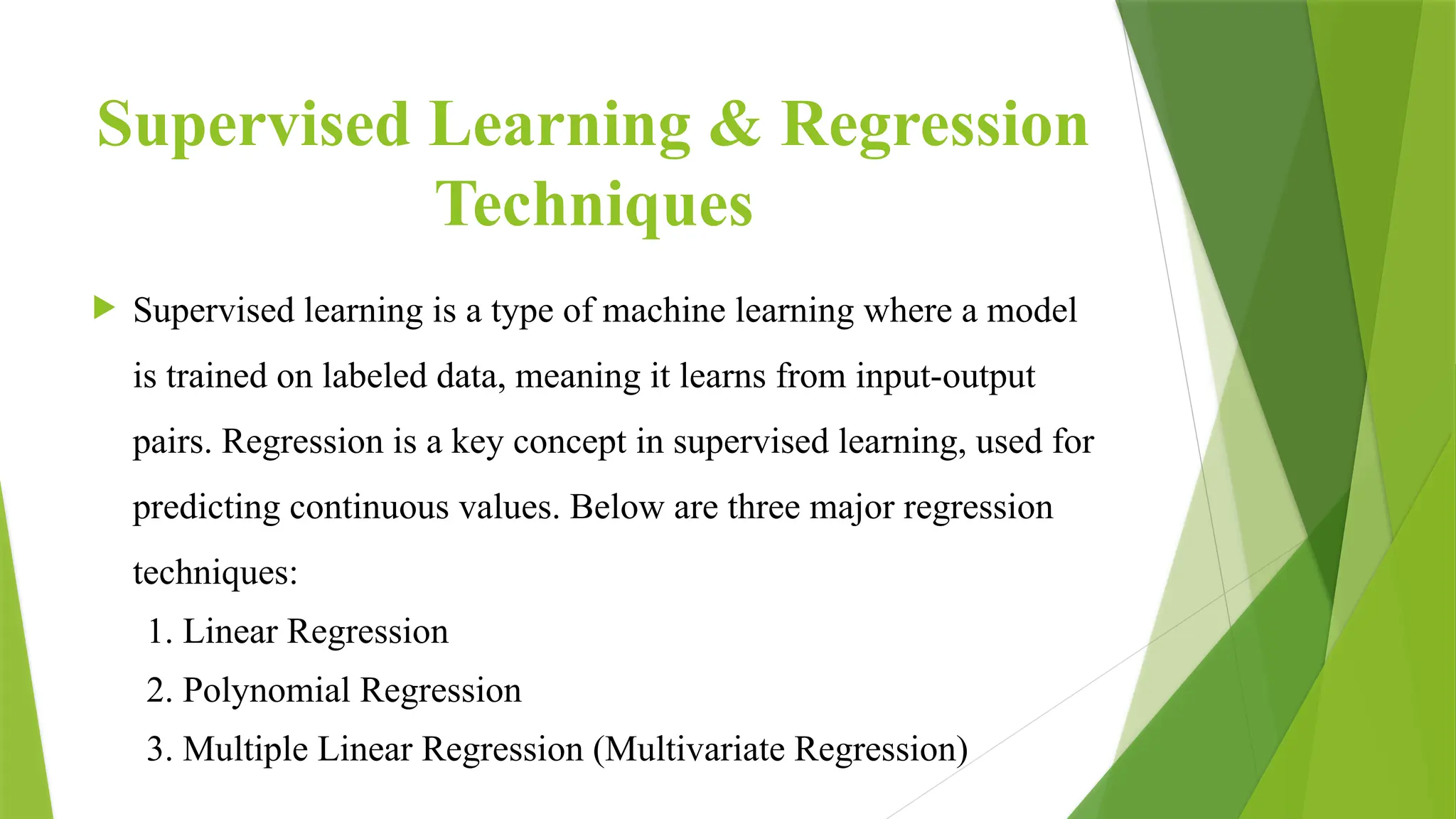
 Supervised learning is a type of machine learning where a model
is trained on labeled data, meaning it learns from input-output
pairs. Regression is a key concept in supervised learning, used for
predicting continuous values. Below are three major regression
techniques:
1. Linear Regression
2. Polynomial Regression
3. Multiple Linear Regression (Multivariate Regression)

3. Linear Regression
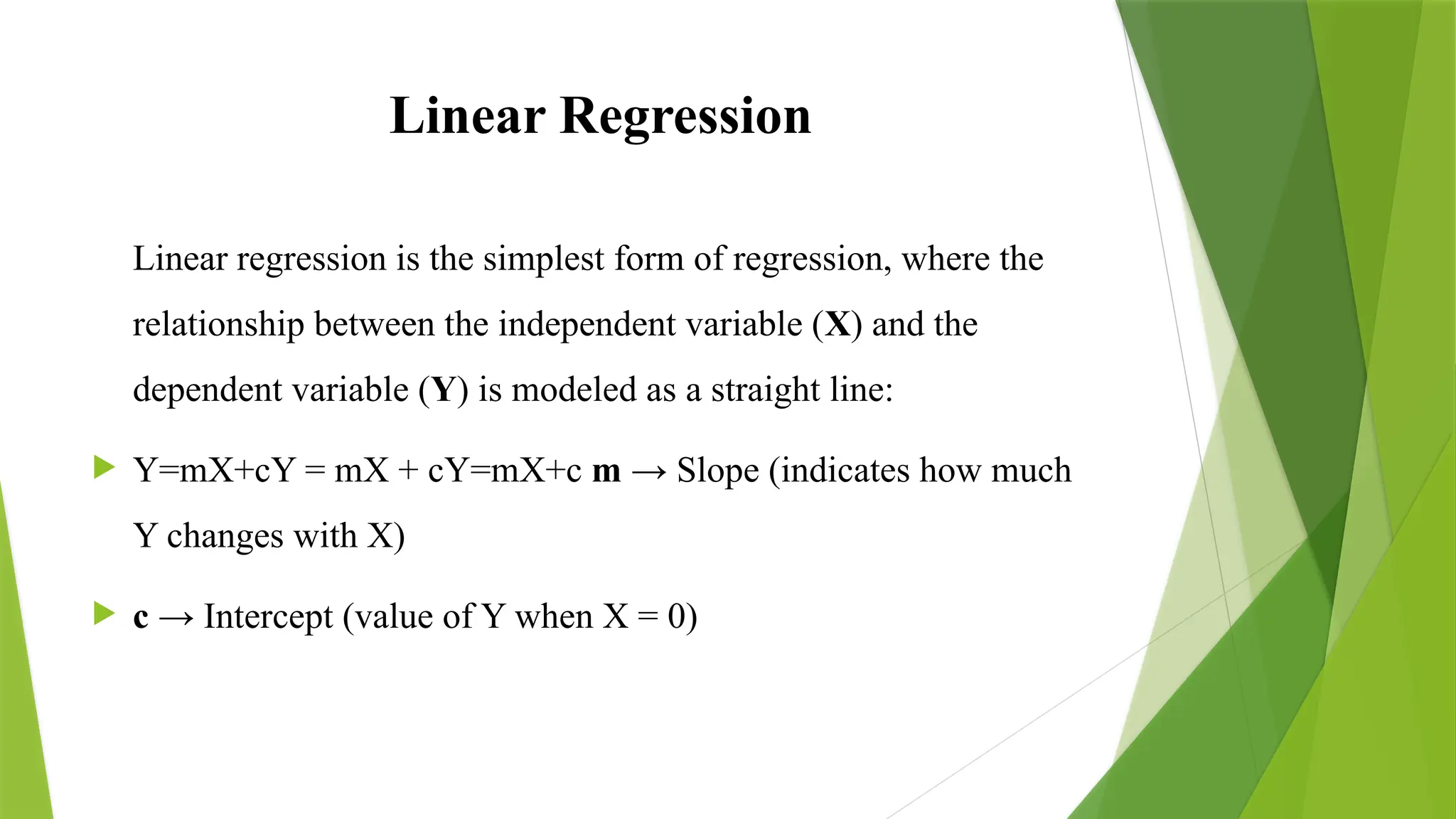
Linear regression is the simplest form of regression, where the
relationship between the independent variable (X) and the
dependent variable (Y) is modeled as a straight line:
 Y=mX+cY = mX + cY=mX+c m → Slope (indicates how much
Y changes with X)
 c → Intercept (value of Y when X = 0)

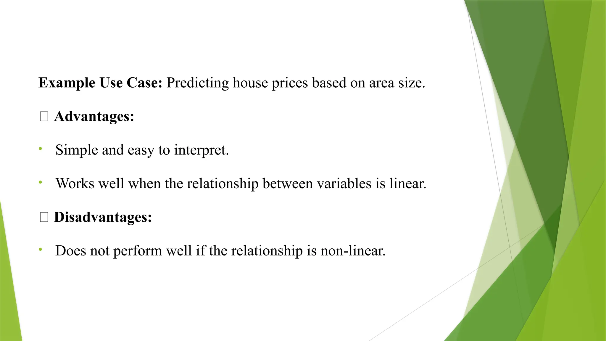
4. Example Use Case: Predicting house prices based on area size.
✅ Advantages:
• Simple and easy to interpret.
• Works well when the relationship between variables is linear.
❌ Disadvantages:
• Does not perform well if the relationship is non-linear.

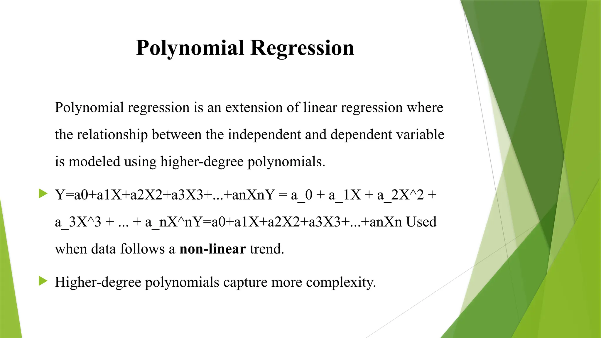
5. Polynomial Regression
Polynomial regression is an extension of linear regression where
the relationship between the independent and dependent variable
is modeled using higher-degree polynomials.
 Y=a0+a1X+a2X2+a3X3+...+anXnY = a_0 + a_1X + a_2X^2 +
a_3X^3 + ... + a_nX^nY=a0​
+a1​
X+a2​
X2+a3​
X3+...+an​
Xn Used
when data follows a non-linear trend.
 Higher-degree polynomials capture more complexity.

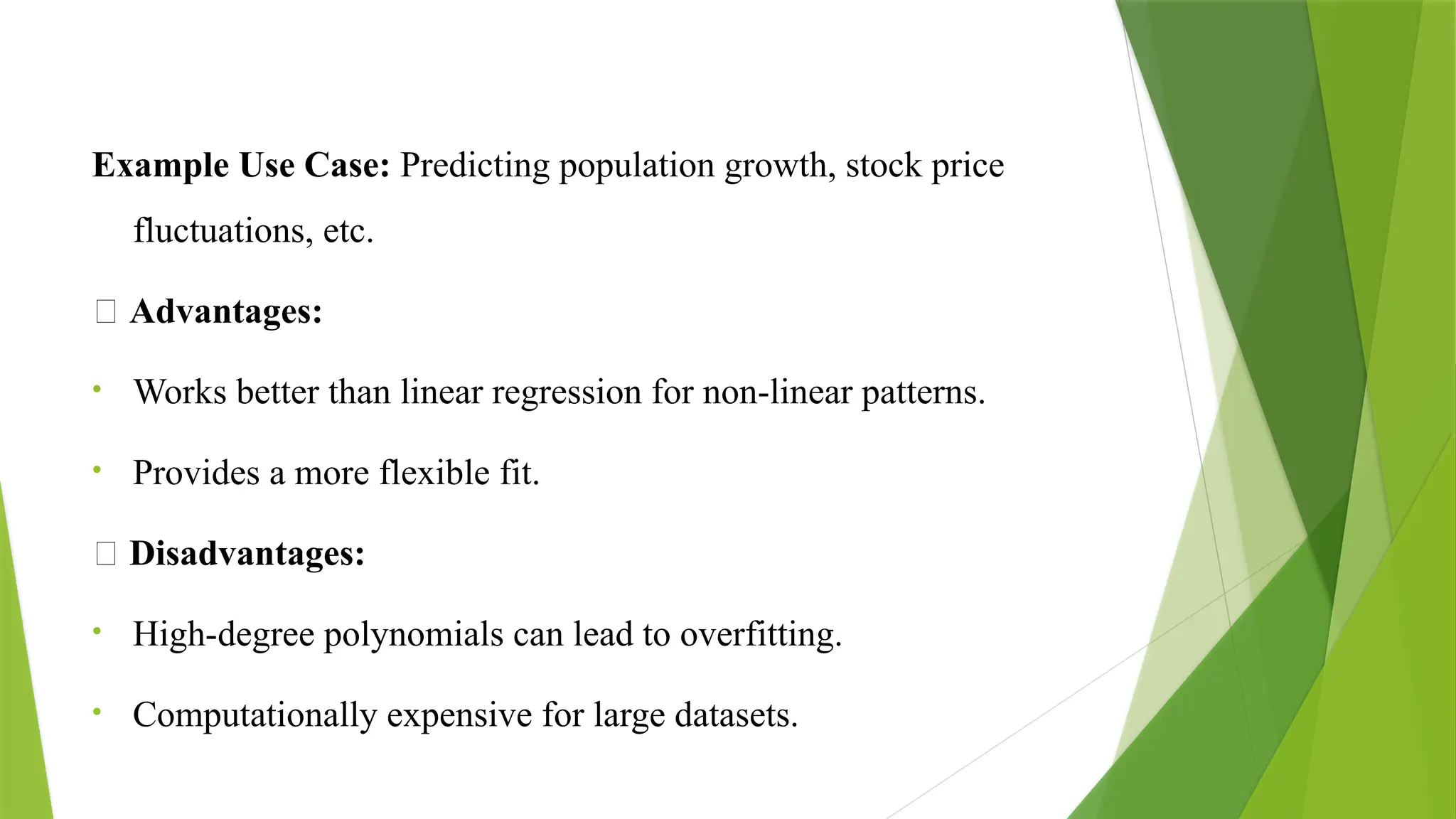
6. Example Use Case: Predicting population growth, stock price
fluctuations, etc.
✅ Advantages:
• Works better than linear regression for non-linear patterns.
• Provides a more flexible fit.
❌ Disadvantages:
• High-degree polynomials can lead to overfitting.
• Computationally expensive for large datasets.

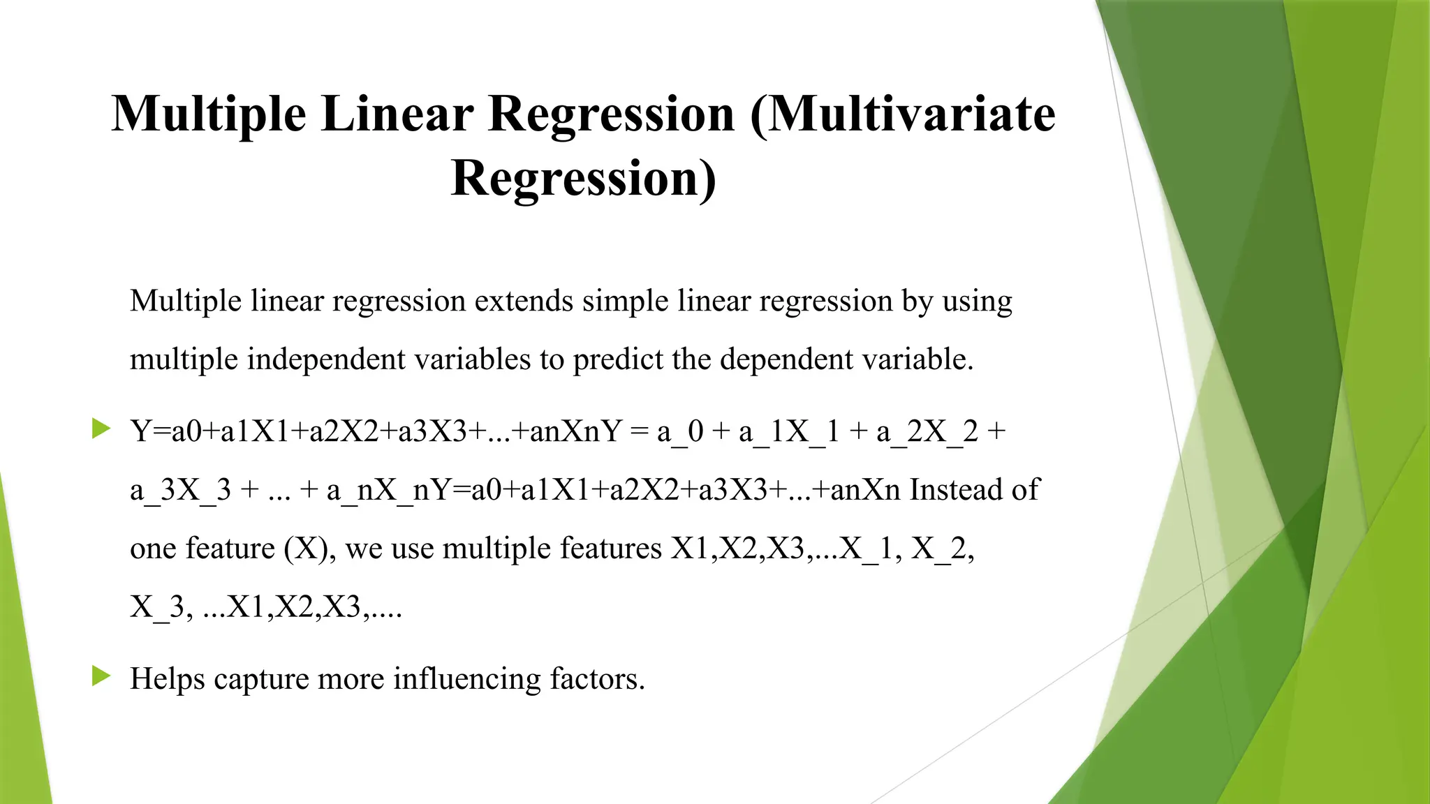
7. Multiple Linear Regression (Multivariate
Regression)
Multiple linear regression extends simple linear regression by using
multiple independent variables to predict the dependent variable.
 Y=a0+a1X1+a2X2+a3X3+...+anXnY = a_0 + a_1X_1 + a_2X_2 +
a_3X_3 + ... + a_nX_nY=a0​
+a1​
X1​
+a2​
X2​
+a3​
X3​
+...+an​
Xn​Instead of
one feature (X), we use multiple features X1,X2,X3,...X_1, X_2,
X_3, ...X1​
,X2​
,X3​
,....
 Helps capture more influencing factors.

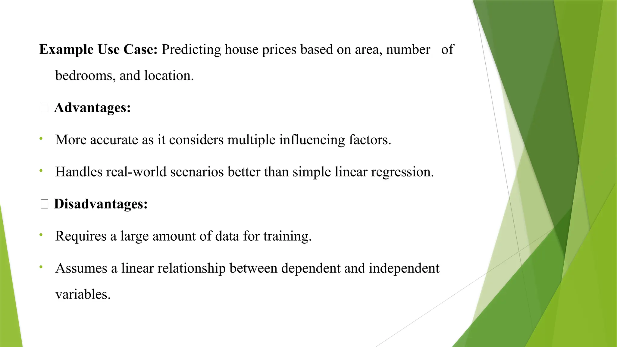
8. Example Use Case: Predicting house prices based on area, number of
bedrooms, and location.
✅ Advantages:
• More accurate as it considers multiple influencing factors.
• Handles real-world scenarios better than simple linear regression.
❌ Disadvantages:
• Requires a large amount of data for training.
• Assumes a linear relationship between dependent and independent
variables.

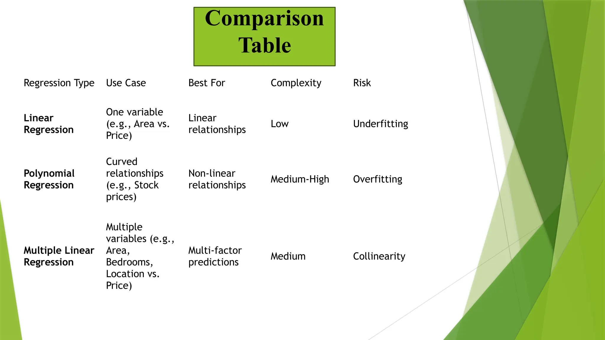
9. Regression Type Use Case Best For Complexity Risk
Linear
Regression
One variable
(e.g., Area vs.
Price)
Linear
relationships
Low Underfitting
Polynomial
Regression
Curved
relationships
(e.g., Stock
prices)
Non-linear
relationships
Medium-High Overfitting
Multiple Linear
Regression
Multiple
variables (e.g.,
Area,
Bedrooms,
Location vs.
Price)
Multi-factor
predictions
Medium Collinearity
Comparison
Table

10. THANK YOU